Databricks

We started Databricks in 2013 in a tiny little office in Berkeley with the belief that data has the potential to solve the world’s toughest problems. We entered 2020 as a global organization with over 1000 employees and a customer base spanning from two-person startups to Fortune 10s.

In this blog post, let’s take a moment to look back and reflect on what we have achieved together in 2019. We will elaborate on the following themes: Solving the World’s Toughest Data Problems, New Developments in the Open Source Ecosystem, and how we are bridging the two with Databricks Platform enhancements.

Databricks Unified Data Analytics Platform

Closing Thoughts

Solve the World’s Toughest Problems

As every year goes by, we encounter more use cases that reinforce our belief that leveraging data effectively is having a profound impact across all industries and disciplines, and we are proud of our part in this journey.

Thousands of organizations have entrusted Databricks with their mission-critical workloads, and have presented their progress at various conferences to disseminate best practices. Some great examples in 2019 include:

Regeneron is able to analyze a massive corpus of genomics data and through machine learning was able to identify a portion of the genome that is responsible for chronic liver disease. By being able to process all of this data quickly, they are now able to create and test a potentially life-saving drug to fight chronic liver disease.
FINRA is able to combat fraud by building a multi-petabyte graph using GraphFrames and then use machine learning to determine which part of graphs have clicks that point to market manipulation.
Quby: Using Europe’s largest energy dataset, consisting of petabytes of IoT data, Quby has developed AI-powered products that are used by hundreds of thousands of users on a daily basis. To learn more about how Quby is conserving the planet, check out Saving Energy in Homes with a Unified Approach to Data and AI.

New Developments in the Open Source Ecosystem

At Spark + AI Summit EU 2019 in Amsterdam, we were excited to announce that the next major version of Apache Spark — Apache Spark 3.0 which includes GPU-aware scheduling — will be released in 2020 as noted in the session New Developments in the Open Source Ecosystem: Apache Spark 3.0, Delta Lake, and Koalas.

The growing Apache Spark ecosystem, including Spark 3.0, Delta Lake, and Koalas

Open Source Delta Lake Project

Delta Lake is an open-source storage layer that brings reliability to data lakes. Delta Lake provides ACID transactions, scalable metadata handling, and unifies streaming and batch data processing. Delta Lake runs on top of your existing data lake and is fully compatible with Apache Spark APIs.

The project has been deployed at thousands of organizations and processes more exabytes of data each week, becoming an indispensable pillar in data and AI architectures. More than 75% of the data scanned on the Databricks Platform is on Delta Lake!

Earlier in 2019, we announced that we were open sourcing the Delta Lake project as noted in the Spark + AI Summit 2019 keynote. Throughout the year, we quickly progressed from version 0.1.0 (April 2019) to version 0.5.0 (December 2019).

Some highlights include:

For a more comprehensive list of how-to blogs, webinars, and meetups and events, refer to the Delta Lake Newsletter (October 2019 edition).

To try out Delta Lake now, a great resource is the Spark + AI Summit EU 2019 tutorial: Building Data-Intensive Analytics Application on Top of Delta Lake.

Easily Scale pandas with Koalas!

For data scientists who love working with the pandas but need to scale, we announced the Koalas open source project. Koalas allows data scientists to easily transition from small datasets to big data by providing a pandas API on Apache Spark.

Even though this project started in early 2019, koalas now has 20,000 downloads per day!

As highlighted in the blog post How Virgin Hyperloop One reduced processing time from hours to minutes with Koalas:

By making changes to less than 1% of our pandas lines, we were able to run our code with Koalas and Spark. We were able to reduce the execution times by more than 10x, from a few hours to just a few minutes, and since the environment is able to scale horizontally, we’re prepared for even more data.

Simplifying Machine Learning Workflows

Introduced in 2018, the MLflow project has the ability to track metrics, parameters, and artifacts as part of experiments, package models and reproducible ML projects, and deploy models to batch or real-time serving platforms.

In 2019, the MLflow project has over 1 million downloads per month!

To help simplify machine learning model workflows, in Fall 2019, we introduced the MLflow Model Registry which builds on MLflow’s existing capabilities to provide organizations with one central place to share ML models, collaborate on moving them from experimentation to testing and production, and implement approval and governance workflows.

Databricks Unified Analytics Platform

The Databricks Unified Analytics Platform is a cloud platform for massive scale data engineering and collaborative data science.

In 2019, the Databricks Unified Data Analytics Platform has created more than one million virtual machines (VMs) every day!

We expanded the Databricks platform with many new features! The full list is quite extensive and can be found in the Databricks Platform Release Notes (AWS | Azure).

Optimizing Storage

In Databricks Runtime 6.0, we enhanced the FUSE mount that enables local file APIs to significantly improve read and write speed as well as support files that are larger than 2 GB. If you need faster and more reliable reads and writes such as for distributed model training, you would find this enhancement particularly useful. For example, as noted in this Spark+AI Summit 2019 session Simplify Distributed TensorFlow Training for Fast Image Categorization at Starbucks, the training of a simple CNN model improved by more than 10x (from 2.62min down to 14.65s).

Databricks Pools

Recently, we launched Databricks pools to speed up your data pipelines and scale clusters quickly. Databricks pools is a managed cache of VM instances that allow you to achieve a reduction in cluster start and auto-scaling times from minutes to seconds!

As well, in 2019 we introduced more regions that are available to use Databricks. As of the end of 2019, there are 29 regions available in Azure and 13 regions in AWS with more coming in 2020!

Databricks Runtime and Databricks Runtime for Machine Learning

In 2019, Databricks Runtime (DBR) for Machine Learning became generally available! As of December 2019, there is DBR 6.2 GA, DBR 6.2 ML, and DBR 6.2 for Genomics. Every DBR release has been tested and verified for version compatibility thus simplifying the management of the different versions of TensorFlow, TensorBoard, PyTorch, Horovod, XGBoost, MLflow, Hyperopt, MLeap, etc.

To simplify Python library and environment management, we also introduced Databricks Runtime with Conda (Beta) Many of our Python users prefer to manage their Python environments and libraries with Conda, which quickly is emerging as a standard. Conda takes a holistic approach to package management by enabling:

The creation and management of environments
Installation of Python packages
Easily reproducible environments
Compatibility with pip

Databricks Runtime with Conda (AWS | Azure) provides an updated and optimized list of default packages and a flexible Python environment for advanced users who require maximum control over packages and environments.

Automatic Logging for Managed MLflow

Managed MLflow on Databricks offers a hosted version of MLflow fully integrated with Databricks’ security model, interactive workspace, and MLflow Sidebar for Databricks Enterprise Edition and Databricks Community Edition.

With Managed MLflow, it is now even easier for data scientists to track their machine learning training sessions for Apache Spark MLlib, Hyperopt, Keras, and Tensorflow without having to change any of their training code.

Augmenting Machine Learning with Databricks Labs’ AutoML Toolkit

Note: The Databricks Labs’ AutoML Toolkit is a labs project to accelerate use cases on the Databricks Unified Analytics Platform.

As mentioned in the Spark+AI Summit Europe 2019 session Augmenting Machine Learning with Databricks Labs AutoML Toolkit, you can significantly streamline the process to build, evaluate, and optimize Machine Learning models by using the Databricks Labs AutoML Toolkit. Using the AutoML Toolkit also allows you to deliver results significantly faster because it allows you to automate the various Machine Learning pipeline stages.

We further simplified the AutoML Toolkit by releasing the AutoML FamilyRunner allowing you to test with a family of different ML algorithms as noted in Using AutoML Toolkit’s FamilyRunner Pipeline APIs to Simplify and Automate Loan Default Predictions.

Closing Thoughts

2019 has been a great year at Databricks! In November 2019, we hired our 1,000th full-time employee. A lot has changed since our first year (2013), you can read more about it in Celebrating Growth at Databricks and 1,000 Employees!

Databricks celebrates its 2019 growth and reaching the 1,000 employee milestone

As part of our amazing growth in 2019, we had both our Series E Funding (February 5th, 2019) and Series F Funding (October 22nd, 2019) with a $6.2 billion valuation! We are setting aside a €100 million ($110 million) slice of the Series F to expand the Amsterdam-based European development center. And at the end of the year, we announced that we were opening up our Databricks engineering office in Toronto in 2020!

This year (2020) will be an even more exciting year with the upcoming Apache Spark 3.0 release and our continued enhancements to Delta Lake, MLflow, Koalas, AutoML, and more! If you’re interested, find your place in Databricks!

Try Databricks for free. Get started today.

The post Solving the World’s Toughest Problems with the Growing Open Source Ecosystem and Databricks appeared first on Databricks.

Try this time series forecasting notebook in Databricks

Advances in time series forecasting are enabling retailers to generate more reliable demand forecasts. The challenge now is to produce these forecasts in a timely manner and at a level of granularity that allows the business to make precise adjustments to product inventories. Leveraging Apache Spark™ and Facebook Prophet, more and more enterprises facing these challenges are finding they can overcome the scalability and accuracy limits of past solutions.

In this post, we’ll discuss the importance of time series forecasting, visualize some sample time series data, then build a simple model to show the use of Facebook Prophet. Once you’re comfortable building a single model, we’ll combine Prophet with the magic of Apache Spark™ to show you how to train hundreds of models at once, allowing us to create precise forecasts for each individual product-store combination at a level of granularity rarely achieved until now.

Accurate and timely forecasting is now more important than ever

Improving the speed and accuracy of time series analyses in order to better forecast demand for products and services is critical to retailers’ success. If too much product is placed in a store, shelf and storeroom space can be strained, products can expire, and retailers may find their financial resources are tied up in inventory, leaving them unable to take advantage of new opportunities generated by manufacturers or shifts in consumer patterns. If too little product is placed in a store, customers may not be able to purchase the products they need. Not only do these forecast errors result in an immediate loss of revenue to the retailer, but over time consumer frustration may drive customers towards competitors.

New expectations require more precise time series models and forecasting methods

For some time, enterprise resource planning (ERP) systems and third-party solutions have provided retailers with demand forecasting capabilities based upon simple time series models. But with advances in technology and increased pressure in the sector, many retailers are looking to move beyond the linear models and more traditional algorithms historically available to them.

New capabilities, such as those provided by Facebook Prophet, are emerging from the data science community, and companies are seeking the flexibility to apply these machine learning models to their time series forecasting needs.

Facebook Prophet logo

This movement away from traditional forecasting solutions requires retailers and the like to develop in-house expertise not only in the complexities of demand forecasting but also in the efficient distribution of the work required to generate hundreds of thousands or even millions of machine learning models in a timely manner. Luckily, we can use Spark to distribute the training of these models, making it possible to predict not just overall demand for products and services, but the unique demand for each product in each location.

Visualizing demand seasonality in time series data

To demonstrate the use of Prophet to generate fine-grained demand forecasts for individual stores and products, we will use a publicly available data set from Kaggle. It consists of 5 years of daily sales data for 50 individual items across 10 different stores.

To get started, let’s look at the overall yearly sales trend for all products and stores. As you can see, total product sales are increasing year over year with no clear sign of convergence around a plateau.

Next, by viewing the same data on a monthly basis, we can see that the year-over-year upward trend doesn’t progress steadily each month. Instead, we see a clear seasonal pattern of peaks in the summer months, and troughs in the winter months. Using the built-in data visualization feature of Databricks Collaborative Notebooks, we can see the value of our data during each month by mousing over the chart.

At the weekday level, sales peak on Sundays (weekday 0), followed by a hard drop on Mondays (weekday 1), then steadily recover throughout the rest of the week.

Getting started with a simple time series forecasting model on Facebook Prophet

As illustrated in the charts above, our data shows a clear year-over-year upward trend in sales, along with both annual and weekly seasonal patterns. It’s these overlapping patterns in the data that Prophet is designed to address.

Facebook Prophet follows the scikit-learn API, so it should be easy to pick up for anyone with experience with sklearn. We need to pass in a 2 column pandas DataFrame as input: the first column is the date, and the second is the value to predict (in our case, sales). Once our data is in the proper format, building a model is easy:

import pandas as pd
from fbprophet import Prophet

# instantiate the model and set parameters
model = Prophet(
    interval_width=0.95,
    growth='linear',
    daily_seasonality=False,
    weekly_seasonality=True,
    yearly_seasonality=True,
    seasonality_mode='multiplicative'
)

# fit the model to historical data
model.fit(history_pd)

Now that we have fit our model to the data, let’s use it to build a 90 day forecast. In the code below, we define a dataset that includes both historical dates and 90 days beyond, using prophet’s make_future_dataframe method:

future_pd = model.make_future_dataframe(
    periods=90,
    freq='d',
    include_history=True
)

# predict over the dataset
forecast_pd = model.predict(future_pd)

That’s it! We can now visualize how our actual and predicted data line up as well as a forecast for the future using Prophet’s built-in .plot method. As you can see, the weekly and seasonal demand patterns we illustrated earlier are in fact reflected in the forecasted results.

predict_fig = model.plot(forecast_pd, xlabel='date', ylabel='sales')
display(fig)

This visualization is a bit busy. Bartosz Mikulski provides an excellent breakdown of it that is well worth checking out. In a nutshell, the black dots represent our actuals with the darker blue line representing our predictions and the lighter blue band representing our (95%) uncertainty interval.

Training hundreds of time series forecasting models in parallel with Prophet and Spark

Now that we’ve demonstrated how to build a single model, we can use the power of Apache Spark to multiply our efforts. Our goal is to generate not one forecast for the entire dataset, but hundreds of models and forecasts for each product-store combination, something that would be incredibly time consuming to perform as a sequential operation.

Building models in this way could allow a grocery store chain, for example, to create a precise forecast for the amount of milk they should order for their Sandusky store that differs from the amount needed in their Cleveland store, based upon the differing demand at those locations.

How to use Spark DataFrames to distribute the processing of time series data

Data scientists frequently tackle the challenge of training large numbers of models using a distributed data processing engine such as Apache Spark. By leveraging a Spark cluster, individual worker nodes in the cluster can train a subset of models in parallel with other worker nodes, greatly reducing the overall time required to train the entire collection of time series models.

Of course, training models on a cluster of worker nodes (computers) requires more cloud infrastructure, and this comes at a price. But with the easy availability of on-demand cloud resources, companies can quickly provision the resources they need, train their models, and release those resources just as quickly, allowing them to achieve massive scalability without long-term commitments to physical assets.

The key mechanism for achieving distributed data processing in Spark is the DataFrame. By loading the data into a Spark DataFrame, the data is distributed across the workers in the cluster. This allows these workers to process subsets of the data in a parallel manner, reducing the overall amount of time required to perform our work.

Of course, each worker needs to have access to the subset of data it requires to do its work. By grouping the data on key values, in this case on combinations of store and item, we bring together all the time series data for those key values onto a specific worker node.

store_item_history
    .groupBy('store', 'item')
    # . . .

We share the groupBy code here to underscore how it enables us to train many models in parallel efficiently, although it will not actually come into play until we set up and apply a UDF to our data in the next section.

Leveraging the power of pandas user-defined functions (UDFs)

With our time series data properly grouped by store and item, we now need to train a single model for each group. To accomplish this, we can use a pandas User-Defined Function (UDF), which allows us to apply a custom function to each group of data in our DataFrame.

This UDF will not only train a model for each group, but also generate a result set representing the predictions from that model. But while the function will train and predict on each group in the DataFrame independent of the others, the results returned from each group will be conveniently collected into single resulting DataFrame. This will allow us to generate store-item level forecasts but present our results to analysts and managers as a single output dataset.

As you can see in the abbreviated code below, building our UDF is relatively straightforward. The UDF is instantiated with the pandas_udf method which identifies the schema of the data it will return and the type of data it expects to receive. Immediately following this, we define the function that will perform the work of the UDF.

Within the function definition, we instantiate our model, configure it and fit it to the data it has received. The model makes a prediction, and that data is returned as the output of the function.

@pandas_udf(result_schema, PandasUDFType.GROUPED_MAP)
def forecast_store_item(history_pd):

    # instantiate the model, configure the parameters
    model = Prophet(
        interval_width=0.95,
        growth='linear',
        daily_seasonality=False,
        weekly_seasonality=True,
        yearly_seasonality=True,
        seasonality_mode='multiplicative'
    )

    # fit the model
    model.fit(history_pd)

    # configure predictions
    future_pd = model.make_future_dataframe(
        periods=90,
        freq='d',
        include_history=True
    )

    # make predictions
    results_pd = model.predict(future_pd)

    # . . .

    # return predictions
    return results_pd

Now, to bring it all together, we use the groupBy command we discussed earlier to ensure our dataset is properly partitioned into groups representing specific store and item combinations. We then simply apply the UDF to our DataFrame, allowing the UDF to fit a model and make predictions on each grouping of data.

The dataset returned by the application of the function to each group is updated to reflect the date on which we generated our predictions. This will help us keep track of data generated during different model runs as we eventually take our functionality into production.

from pyspark.sql.functions import current_date

results = (
    store_item_history
    .groupBy('store', 'item')
    .apply(forecast_store_item)
    .withColumn('training_date', current_date())
    )

Next steps

We have now constructed a forecast for each store-item combination. Using a SQL query, analysts can view the tailored forecasts for each product. In the chart below, we’ve plotted the projected demand for product #1 across 10 stores. As you can see, the demand forecasts vary from store to store, but the general pattern is consistent across all of the stores, as we would expect.

As new sales data arrives, we can efficiently generate new forecasts and append these to our existing table structures, allowing analysts to update the business’s expectations as conditions evolve.

Try Databricks for free. Get started today.

The post Fine-Grained Time Series Forecasting At Scale With Facebook Prophet And Apache Spark appeared first on Databricks.

We recently hosted a live webinar — Geospatial Analytics and AI in Public Sector — during which we covered top geospatial analysis use cases in the Public Sector along with live demos showcasing how to build scalable analytics and machine learning pipelines on geospatial data at sale.

Geospatial Analytics Webinar Overview

Today, government agencies have access to massive volumes of geospatial information that can be analyzed to deliver on a broad range of decision-making and predictive analytics use cases from transportation planning to disaster recovery and population health management.

While many agencies have invested in geographic information systems that produce volumes of geospatial data, few have the proper technology and technical expertise to prepare these large, complex datasets for analytics — inhibiting their ability to build AI applications.

In this webinar, we reviewed:

Top geospatial big data use cases in Public Sector spanning public safety, defense, infrastructure management, health services, fraud prevention and more
Challenges analyzing large volumes of geospatial data with legacy architectures
How Databricks and open-source tools can be used to overcome these challenges in the cloud
Technical demos and notebooks shared on the webinar:

Object Detection in xView Imagery: Bridges complex object detection using Deep Learning with accessible SQL-based analytics for non-data scientist personas. Download related notebooks: data engineering and analysis.
Processing Large-Scale NYC Taxi Pickup / Dropoff Vectors: Optimizes geospatial predicate operations and joins to associate raw pick-up/drop-off coordinates with their corresponding NYC neighborhood boundaries to facilitate spatial analysis. Download related notebook.

If you’d like free access to the Unified Data Analytics Platform and try our notebooks on it, you can access a free Databricks trial here.

At the end of the webinar we held a Q&A. Below are the questions and answers:

Q: We deal with large volumes of streaming geospatial data. How would you recommend handling these real-time data streams for downstream analytics?

A: This can be broken down to (1) handling large volumes of streaming data and (2) performing downstream geospatial analytics. Databricks makes processing and storing large volumes of streaming data simple, reliable, and performant. Please reference Delta Lake on Databricks and Introduction to Delta Lake for some additional material. The second part builds on storage and schema decisions made during the processing phase. Spatial analysis is fundamentally addressed through the use of Spark SQL, DataFrames, and Datasets to power transformations and actions over data originating from various formats and schemas. Databricks offers various runtimes such as Machine Learning Runtime and Databricks Runtime with Conda which pre-bundle popular libraries including Tensorflow, Horovod, PyTorch, Scikit-Learn, and Anaconda for both CPU and GPU clusters to facilitate common Data Engineering and Data Science needs. Customers can also manage their own Libraries or Containers to customize the environment for any analytic, to include spatial specific needs. Please reference popular spatial frameworks listed in the following question as well as the FINRA Customer Case Study

Q: What are some of the more popular spatial frameworks being used in the public sector?

A: Popular frameworks which extend Apache Spark for geospatial analytics include GeoMesa, GeoTrellis, Rasterframes, and GeoSpark. In addition, Databricks makes it easy to use single-node libraries such as GeoPandas, Shapely, Geospatial Data Abstraction Library (GDAL), and Java Topology Service (JTS). By wrapping function calls in user-defined functions (UDFs) these libraries can further be leveraged in a distributed context as well. UDFs offer a simple approach for scaling existing workloads with minimal code changes.

Q: Where is my data stored and how does Databricks help ensure data security?

A: Your data is stored in your own cloud data lake, such as in AWS S3 or Azure Blob Storage. However, data lakes often have data quality issues, due to a lack of control over ingested data. Delta Lake adds a storage layer to data lakes to manage data quality, ensuring data lakes contain only high-quality data for consumers. Delta Lake also offers capabilities like ACID transactions to ensure data integrity with serializability as well as audit history, allowing you to maintain log records details about every change made to data, providing a full history of changes, for compliance, audit, and reproduction. Additionally, Delta Lake has been designed to address various right-to-erasure initiatives such as the General Data Protection Regulation (GDPR) and recently the California Consumer Privacy Act (CCPA), reference Make Your Data Lake CCPA Compliant with a Unified Approach to Data and Analytics. As part of our Enterprise Cloud Service, Delta Lake is tightly integrated with other Databricks Enterprise Security features.

Additional Geospatial Analytics Resources

Sign-up for a free trial and download these notebooks to start experimenting:

Read our recent blog Processing Geospatial Data at Scale With Databricks to learn how Databricks Unified Data Analytics Platform addresses challenges around ingesting, storing, and analyzing spatial data of massive size
Download our Guide to Data Analytics and AI at Scale for the Public Sector
Visit our Public Sector page to learn how the Center for Medicare & Medicaid Services, DHS and other agencies are innovating with Databricks

Try Databricks for free. Get started today.

The post On-Demand Webinar: Geospatial Analytics and AI in the Public Sector appeared first on Databricks.

We are excited to announce the release of Delta Lake 0.5.0, which introduces Presto/Athena support and improved concurrency.

The key features in this release are:

Support for other processing engines using manifest files (#76) – You can now query Delta tables from Presto and Amazon Athena using manifest files, which you can generate using Scala, Java, Python, and SQL APIs. See the Presto and Athena to Delta Lake Integration documentation for details
Improved concurrency for all Delta Lake operations (#9, #72, #228) – You can now run more Delta Lake operations concurrently. Delta Lake’s optimistic concurrency control has been improved by making conflict detection more fine-grained. This makes it easier to run complex workflows on Delta tables. For example:
- Running deletes (e.g. for GDPR compliance) concurrently on older partitions while newer partitions are being appended.
- Running updates and merges concurrently on disjoint sets of partitions.
- Running file compactions concurrently with appends (see below).

For more information, please refer to the open-source Delta Lake 0.5.0 release notes. In this blog post, we will elaborate on reading Delta Lake tables with Presto, improved operations concurrency, easier and faster data deduplication using insert-only merge.

Reading Delta Lake Tables with Presto

As described in Simple, Reliable Upserts and Deletes on Delta Lake Tables using Python APIs, modifications to the data such as deletes are performed by selectively writing new versions of the files containing the data be deleted and only marks the previous files as deleted. The advantage of this approach is that Delta Lake enables us to travel back in time (i.e. time travel) and query previous versions.

To understand which files (and rows) contain the latest data, by default you can query the transaction log (more information at Diving Into Delta Lake: Unpacking The Transaction Log). Other systems like Presto and Athena can read a generated manifest file – a text file containing the list of data files to read for querying a table. To do this, we will follow the Python instructions; for more information, refer to Set up the Presto or Athena to Delta Lake integration and query Delta tables.

Generate Delta Lake Manifest File

Let’s start by creating the Delta Lake manifest file with the following code snippet.

deltaTable = DeltaTable.forPath(pathToDeltaTable)
deltaTable.generate("symlink_format_manifest")

As the name implies, this generates the manifest file in the table root folder. If you had created the departureDelays table per Simple, Reliable Upserts and Deletes on Delta Lake Tables using Python APIs, you will have a new folder in the table root folder:

$/departureDelays.delta/_symlink_format_manifest

with a single file named manifest. If you review the files within the manifest (e.g. cat manifest), you will get the following output indicating the files that contain the latest snapshot.

file:$/departureDelays.delta/part-00003-...-c000.snappy.parquet
file:$/departureDelays.delta/part-00006-...-c000.snappy.parquet
file:$/departureDelays.delta/part-00001-...-c000.snappy.parquet
file:$/departureDelays.delta/part-00000-...-c000.snappy.parquet
file:$/departureDelays.delta/part-00000-...-c000.snappy.parquet
file:$/departureDelays.delta/part-00001-...-c000.snappy.parquet
file:$/departureDelays.delta/part-00002-...-c000.snappy.parquet
file:$/departureDelays.delta/part-00007-...-c000.snappy.parquet

Create Presto Table to Read Generated Manifest File

The next step is to create an external table in the Hive Metastore so that Presto (or Athena with Glue) can read the generated manifest file to identify which Parquet files to read for reading the latest snapshot of the Delta table. Note, for Presto, you can either use Apache Spark or the Hive CLI to run the following command. k.

1. CREATE EXTERNAL TABLE departureDelaysExternal ( ... )
2. ROW FORMAT SERDE
   'org.apache.hadoop.hive.ql.io.parquet.serde.ParquetHiveSerDe'
3. STORED AS INPUTFORMAT
4. OUTPUTFORMAT
   'org.apache.hadoop.hive.ql.io.HiveIgnoreKeyTextOutputFormat'
5. LOCATION '$/departureDelays.delta/_symlink_format_manifest'

Some important notes on schema enforcement:

The schema defined on line 1 must match the schema of the Delta Lake table (e.g. in this example, departureDelaysExternal). Note, the partitioning scheme is optional.
Line 5 points to the location of the manifest file in the form of /_symlink_format_manifest/

The SymlinkTextInputFormat configures Presto (or Athena) to get the list of Parquet data files from the manifest file instead of using directory listing. Note, for partitioned tables, there are additional steps that will need to be performed per Configure Presto to read the generated manifests.

Update the Manifest File

It is important to note that every time the data is updated, you will need to regenerate the manifest file so Presto will be able to see the latest data.

Improved Operations Concurrency

With the following pull requests, you can now run even more Delta Lake operations concurrently. With finer grain conflict detection, these updates make it easier to run complex workflows on Delta tables such as:

Running deletes (e.g. for GDPR compliance) concurrently on older partitions while newer partitions are being appended.
Running file compactions concurrently with appends.
Running updates and merges concurrently on disjoint sets of partitions.

Concurrent Appends Use Cases

For example, typically there is a ConcurrentAppendException thrown during concurrent merge operations when concurrent transaction adds records to the same partition.

// Target 'deltaTable' is partitioned by date and country
deltaTable.as("t").merge(
    source.as("s"),
    "s.user_id = t.user_id AND s.date = t.date AND s.country = t.country")
  .whenMatched().updateAll()
  .whenNotMatched().insertAll()
  .execute()

The above code snippet potentially can cause conflicts because the condition is not explicit enough resulting even though the table is already partitioned by date and country. The issue is that the query currently will scan the entire table potentially resulting in a conflict with concurrent operations updating any other partitions. By specifying specificDate and specificCountry so you can merge on a specific date or country, this operation is now safe to run concurrently on different dates and countries.

// Target 'deltaTable' is partitioned by date and country
deltaTable.as("t").merge(
    source.as("s"),
    "s.user_id = t.user_id AND d.date = '" + specificDate + "' AND d.country = '" + specificCountry + "'")
  .whenMatched().updateAll()
  .whenNotMatched().insertAll()
  .execute()

This approach is the same for all other Delta Lake operations (e.g. delete, metadata changed, etc.).

Concurrent File Compaction

If you are continuously writing data to a Delta table, over time a large number of files will be accumulated. This is especially important in streaming scenarios as you are adding data in small batches. This results in the file system continuing to accumulate many small files; this will degrade query performance over time. An important optimization task is to periodically take a large number of small files and rewrite them to a smaller number of larger files, i.e. file compaction.

In the past, there was a higher potential for an exception when concurrently querying the data and running file compaction. But, because of these improvements, you can also run queries (including streaming queries) and file compaction concurrently without any exceptions. For example, If your table is partitioned and you want to repartition just one partition based on a predicate, you can read only the partition using where and write back to that using replaceWhere:

path = "..."
partition = "year = '2019'"
numFilesPerPartition = 16   # Compact partition of a table to no. of files

(spark.read
  .format("delta")
  .load(path)
  .where(partition)
  .repartition(numFilesPerPartition)
  .write
  .option("dataChange", "false")
  .format("delta")
  .mode("overwrite")
  .option("replaceWhere", partition)
  .save(path))

Note, use the dataChange == false option only when there are no data changes (such as in the preceding code snippet) otherwise this may corrupt the underlying data.

Easier and Faster Data Deduplication Using Insert-only Merge

A common ETL use case is to collect logs and append them into a Delta Lake table. A common issue is that the source generates duplicate log records. With Delta Lake merge, you can avoid inserting these duplicate records such as the following code snippet involving merging updated flight data.

# Merge merge_table with flights
deltaTable.alias("flights") \
    .merge(merge_table.alias("updates"),"flights.date = updates.date") \
    .whenMatchedUpdate(set = { "delay" : "updates.delay" } ) \
    .whenNotMatchedInsertAll() \
    .execute()

Prior to Delta Lake 0.5.0, it was not possible to read deduped data as a stream from a Delta Lake table because insert-only merges were not pure appends into the table.

For example, in a streaming query, you can run a merge operation in foreachBatch to continuously write any streaming data into a Delta Lake table with deduplication as noted in the following PySpark snippet.

from delta.tables import *

deltaTable = DeltaTable.forPath(spark, "/data/aggregates")

# Function to upsert microBatchOutputDF into Delta table using merge
def upsertToDelta(microBatchOutputDF, batchId):
  deltaTable.alias("t").merge(
      microBatchOutputDF.alias("s"),
      "s.key = t.key") \
    .whenMatchedUpdateAll() \
    .whenNotMatchedInsertAll() \
    .execute()
}

# Write the output of a streaming aggregation query into Delta table
streamingAggregatesDF.writeStream \
  .format("delta") \
  .foreachBatch(upsertToDelta) \
  .outputMode("update") \
  .start()

In another streaming query, you can continuously read deduplicated data from this Delta Lake table. This is possible because insert-only merge – introduced in Delta Lake 0.5.0 – will only append new data to the Delta table.

Getting Started with Delta Lake 0.5.0

Try out Delta Lake today by trying out the preceding code snippets on your Apache Spark 2.4.3 (or newer) instance. By using Delta Lake, you can make your data lakes more reliable (whether you create a new one or migrate an existing data lake). To learn more, refer to https://delta.io/ and join the Delta Lake open source community via Slack and Google Group. You can track all the upcoming releases and planned features in Delta Lake github milestones.

Credits

We want to thank the following contributors for updates, doc changes, and contributions in Delta Lake 0.5.0: Andreas Neumann, Andrew Fogarty, Burak Yavuz, Denny Lee, Fabio B. Silva, JassAbidi, Matthew Powers, Mukul Murthy, Nicolas Paris, Pranav Anand, Rahul Mahadev, Reynold Xin, Shixiong Zhu, Tathagata Das, Tomas Bartalos, and Xiao Li.

Try Databricks for free. Get started today.

The post Query Delta Lake Tables from Presto and Athena, Improved Operations Concurrency, and Merge performance appeared first on Databricks.

Over the past few years at Databricks, we’ve seen a new data management paradigm that emerged independently across many customers and use cases: the data lakehouse. In this post we describe this new system and its advantages over previous technologies.

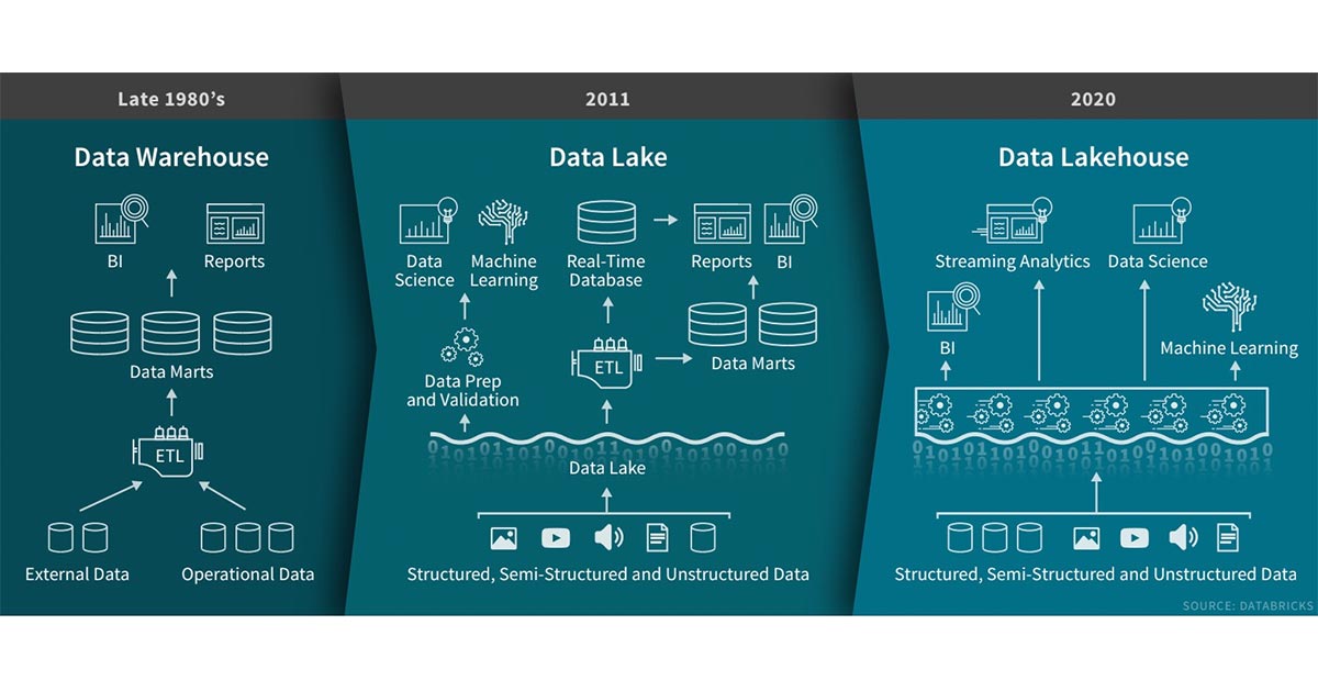
Data warehouses have a long history in decision support and business intelligence applications. Since its inception in the late 1980s, data warehouse technology continued to evolve and MPP architectures led to systems that were able to handle larger data sizes. But while warehouses were great for structured data, a lot of modern enterprises have to deal with unstructured, semi structured, and data with high variety, velocity, and volume. Data warehouses are not suited for many of these use cases, and they are certainly not the most cost efficient.

As companies began to collect large amounts of data from many different sources, architects began envisioning a single system to house data for many different analytic products and workloads. About a decade ago companies began building data lakes – repositories for raw data in a variety of formats. While suitable for storing data, data lakes lack some critical features: they do not support transactions, they do not enforce data quality, and their lack of consistency / isolation makes it almost impossible to mix appends and reads, and batch and streaming jobs.

The need for a flexible, high-performance system hasn’t abated. Companies require systems for diverse data applications including SQL analytics, real-time monitoring, data science, and machine learning. Most of the recent advances in AI have been in better models to process unstructured data (text, images, video, audio), but these are precisely the types of data that a data warehouse is not optimized for. A common approach is to use multiple systems – a data lake, several data warehouses, and other specialized systems such as streaming, time-series, graph, and image databases. Having a multitude of systems introduces complexity and more importantly, introduces delay as data professionals invariably need to move or copy data between different systems.

Evolution of data storage, from data warehouses to data lakes to data lakehouses

What is a data lakehouse?

New systems are beginning to emerge that address the limitations of data lakes. A data lakehouse is a new paradigm that combines the best elements of data lakes and data warehouses. Data lakehouses are enabled by a new system design: implementing similar data structures and data management features to those in a data warehouse, directly on the kind of low cost storage used for data lakes. They are what you would get if you had to redesign data warehouses in the modern world, now that cheap and highly reliable storage (in the form of object stores) are available.

A data lakehouse has the following key features:

Storage is decoupled from compute: In practice this means storage and compute use separate clusters, thus these systems are able to scale to many more concurrent users and larger data sizes. Some modern data warehouses also have this property.
Openness: The storage formats they use are open and they provide an API so different tools and engines, including machine learning and Python/R libraries, can access data. For example, existing data lakehouses enable using BI tools directly on the source data. This reduces staleness and improves recency, reduces latency, and lowers the cost of having to operationalize two copies of the data in both a data lake and a warehouse.
Support for diverse data types ranging from unstructured to structured data: The data lakehouse supports SQL and can house relational data including star-schemas commonly used in data warehouses. In addition they can be used to store, refine, analyze, and access data types needed for many new data applications, including images, video, audio, semi-structured data, and text.
Support for diverse workloads: including SQL and analytics, data science, and machine learning. Multiple tools might be needed to support all these workloads but they all rely on the same data repository.
Transaction support: In an enterprise data lakehouse many data pipelines will often be reading and writing data concurrently. Support for ACID transactions ensures that as multiple parties concurrently read or write data, the system is able to reason about data integrity.
End-to-end streaming: Real-time reports are the norm in many enterprises. Support for streaming eliminates the need for separate systems dedicated to serving real-time data applications.

These are the key attributes of data lakehouses. Enterprise grade systems require additional features. Tools for security and access control are basic requirements. Data governance capabilities including auditing, retention, and lineage have become essential particularly in light of recent privacy regulations. Tools that enable data discovery such as data catalogs and data usage metrics are also needed. With a data lakehouse, such enterprise features only need to be implemented, tested, and administered for a single system.

Some early examples

The Databricks Platform has the architectural features of a data lakehouse. Microsoft’s Azure Synapse Analytics service, which integrates with Azure Databricks, enables a similar lakehouse pattern. Other managed services such as BigQuery and Redshift Spectrum have some of the lakehouse features listed above, but they are examples that focus primarily on BI and other SQL applications. Companies who want to build and implement their own systems have access to open source file formats (Delta Lake, Apache Iceberg, Apache Hudi) that are suitable for building a data lakehouse.

Merging data lakes and data warehouses into a single system means that data teams can move faster as they are able use data without needing to access multiple systems. The level of SQL support and integration with BI tools among these early data lakehouses are generally sufficient for most enterprise data warehouses. Materialized views and stored procedures are available but users may need to employ other mechanisms that aren’t equivalent to those found in traditional data warehouses. The latter is particularly important for “lift and shift scenarios”, which require systems that achieve semantics that are almost identical to those of older, commercial data warehouses.

What about support for other types of data applications? Users of a data lakehouse have access to a variety of standard tools (Spark, Python, R, machine learning libraries) for non BI workloads like data science and machine learning. Data exploration and refinement are standard for many analytic and data science applications. Delta Lake is designed to let users incrementally improve the quality of data in their lakehouse until it is ready for consumption.

A note about technical building blocks. While distributed file systems can be used for the storage layer, objects stores are more commonly used in data lakehouses. Object stores provide low cost, highly available storage, that excel at massively parallel reads – an essential requirement for modern data warehouses.

From BI to AI

The data lakehouse is a new data management paradigm that radically simplifies enterprise data infrastructure and accelerates innovation in an age when machine learning is poised to disrupt every industry. In the past most of the data that went into a company’s products or decision making was structured data from operational systems, whereas today, many products incorporate AI in the form of computer vision and speech models, text mining, and others. Why use a data lakehouse instead of a data lake for AI? A data lakehouse gives you data versioning, governance, security and ACID properties that are needed even for unstructured data.

Current data lakehouses reduce cost but their performance can still lag specialized systems (such as data warehouses) that have years of investments and real-world deployments behind them. Users may favor certain tools (BI tools, IDEs, notebooks) over others so data lakehouses will also need to improve their UX and their connectors to popular tools so they can appeal to a variety of personas. These and other issues will be addressed as the technology continues to mature and develop. Over time data lakehouses will close these gaps while retaining the core properties of being simpler, more cost efficient, and more capable of serving diverse data applications.

Try Databricks for free. Get started today.

The post What Is a Data Lakehouse? appeared first on Databricks.

With technological advancements in imaging and the availability of new efficient computational tools, digital pathology has taken center stage in both research and diagnostic settings. Whole Slide Imaging (WSI) has been at the center of this transformation, enabling us to rapidly digitize pathology slides into high resolution images. By making slides instantly shareable and analyzable, WSI has already improved reproducibility and enabled enhanced education and remote pathology services.

Today, digitization of entire slides at very high resolution can occur inexpensively in less than a minute. As a result, more and more healthcare and life sciences organizations have acquired massive catalogues of digitized slides. These large datasets can be used to build automated diagnostics with machine learning, which can classify slides—or segments thereof—as expressing a specific phenotype, or directly extract quantitative biomarkers from slides. With the power of machine learning and deep learning thousands of digital slides can be interpreted in a matter of minutes. This presents a huge opportunity to improve the efficiency and effectiveness of pathology departments, clinicians and researchers to diagnose and treat cancer and infectious diseases.

3 Common Challenges Preventing Wider Adoption of Digital Pathology Workflows

While many healthcare and life sciences organizations recognize the potential impact of applying artificial intelligence to whole slide images, implementing an automated slide analysis pipeline remains complex. An operational WSI pipeline must be able to routinely handle a high throughput of digitizer slides at a low cost. We see three common challenges preventing organizations from implementing automated digital pathology workflows with support for data science:

Slow and costly data ingest and engineering pipelines: WSI images are usually very large (typically 0.5–2 GB per slide) and can require extensive image pre-processing.
Trouble scaling deep learning to terabytes of images: Training a deep learning model across a modestly sized dataset with hundreds of WSIs can take days to weeks on a single node. These latences prevent rapid experimentation on large datasets. While latency can be reduced by parallelizing deep learning workloads across multiple nodes, this is an advanced technique that is out of the reach of a typical biological data scientist.
Ensuring reproducibility of the WSI workflow: When it comes to novel insights based on patient data, it is very important to be able to reproduce results. Current solutions are mostly ad-hoc and do not allow efficient ways of keeping track of experiments and versions of the data used during machine learning model training.

In this blog, we discuss how the Databricks Unified Data Analytics Platform can be used to address these challenges and deploy an end-to-end scalable deep learning workflows on WSI image data. We will focus on a workflow that trains an image segmentation model that identifies regions of metastases on a slide. In this example, we will use Apache Spark to parallelize data preparation across our collection of images, use pandas UDF to extract features based on pre-trained models (transfer learning) across many nodes, and MLflow to reproducibly track our model training.

End-to-end Machine Learning on WSI

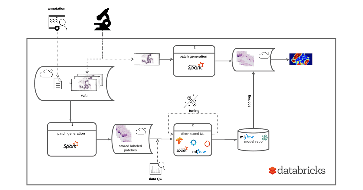
To demonstrate how to use the Databricks platform to accelerate a WSI data processing pipeline, we will use the Camelyon16 Grand Challenge dataset. This is an open-access dataset of 400 whole slide images in TIFF format from breast cancer tissues to demonstrate our workflows. A subset of the Camelyon16 dataset can be directly accessed from Databricks under /databricks-datasets/med-images/camelyon16/ (AWS | Azure). To train an image classifier to detect regions in a slide that contain cancer metastases, we will run the following three steps, as shown in Figure 1:

Patch Generation: Using coordinates annotated by a pathologist, we crop slide images into equally sized patches. Each image can generate thousands of patches, and is labeled as tumor or normal.
Deep Learning: We use transfer learning to use a pre-trained model to extract features from image patches and then use Apache Spark to train a binary classifier to predict tumor vs. normal patches.
Scoring: We then use the trained model that is logged using MLflow to project a probability heat-map on a given slide.

Similar to the workflow Human Longevity used to preprocess radiology images, we will use Apache Spark to manipulate both our slides and their annotations. For model training, we will start by extracting features using a pre-trained InceptionV3 model from Keras. To this end, we leverage Pandas UDFs to parallelize feature extraction. For more information on this technique see Featurization for Transfer Learning (AWS|Azure). Note that this technique is not specific to InceptionV3 and can be applied to any other pre-trained model.

Figure 1: Implementing an end-to-end solution for training and deployment of a DL model based on WSI data

Image Preprocessing and ETL

Using open source tools such as Automated Slide Analysis Platform, pathologists can navigate WSI images at very high resolution and annotate the slide to mark sites that are clinically relevant. The annotations can be saved as an XML file, with the coordinates of the edges of the polygons containing the site and other information, such as zoom level. To train a model that uses the annotations on a set of ground truth slides, we need to load the list of annotated regions per image, join these regions with our images, and excise the annotated region. Once we have completed this process, we can use our image patches for machine learning.

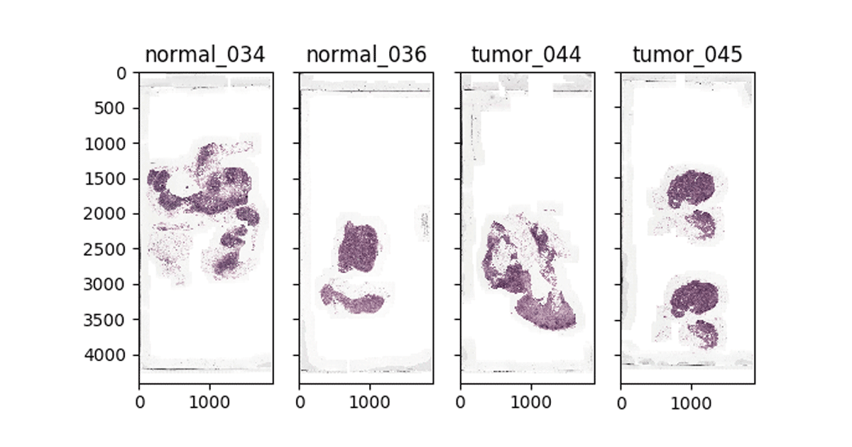
Figure 2: Visualizing WSI images in Databricks notebooks

Although this workflow commonly uses annotations stored in an XML file, for simplicity, we are using the pre-processed annotations made by the Baidu Research team that built the NCRF classifier on the Camelyon16 dataset. These annotations are stored as CSV encoded text files, which Apache Spark will load into a DataFrame. In the notebook cell below, we load the annotations for both tumor and normal patches, and assign the label 0 to normal slices and 1 to tumor slices. We then union the coordinates and labels into a single DataFrame.

While many SQL-based systems restrict you to built-in operations, Apache Spark has rich support for user defined functions (UDFs). UDFs allow you to call a custom Scala, Java, Python, or R function on data in any Apache Spark DataFrame. In our workflow, we will define a Python UDF that uses the OpenSlide library to excise a given patch from an image. We define a python function that takes the name of the WSI to be processed, the X and Y coordinates of the patch center, and the label for the patch and creates tile that later will be used for training.

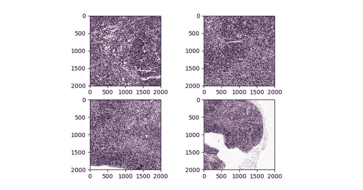
Figure 3. Visualizing patches at different zoom levels

We then use the OpenSlide library to load the images from cloud storage, and to slice out the given coordinate range. While OpenSlide doesn’t natively understand how to read data from Amazon S3 or Azure Data Lake Storage, the Databricks File System (DBFS) FUSE layer allows OpenSlide to directly access data stored in these blob stores without any complex code changes. Finally, our function writes the patch back using the DBFS FUSE layer.

It takes approximately 10 minutes for this command to generate ~174000 patches from the Camelyon16 dataset on databricks datasets. Once our command has completed, we can load our patches back up and display them directly in-line in our notebook.

Training a tumor/normal pathology classifier using transfer learning and MLFlow

In the previous step, we generated patches and associated metadata, and stored generated image tiles using cloud storage. Now, we are ready to train a binary classifier to predict whether a segment of a slide contains a tumor metastasis. To do this, we will use transfer learning to extract features from each patch using a pre-trained deep neural network and then use sparkml for the classification task. This technique frequently outperforms training from scratch for many image processing applications. We will start with the InceptionV3 architecture, using pre-trained weights from Keras.

Apache Spark’s DataFrames provide a built-in Image schema and we can directly load all patches into a DataFrame. We then use Pandas UDFs to transform the images into features based on InceptionV3 using Keras. Once we have featurized each image, we use spark.ml to fit a logistic regression between the features and the label for each patch. We log the logistic regression model with MLFlow so that we can access the model later for serving.

When running ML workflows on Databricks, users can take advantage of managed MLFlow. With every run of the notebook and every training round, MLFlow automatically logs parameters, metrics and any specified artifact. In addition, it stores the trained model that can later be used for predicting labels on data. We refer interested readers to these docs for more information on how MLFlow can be leveraged to manage a full-cycle of ML workflow on databricks.

Table 1 shows the time spent on different parts of the workflow. We notice that the model training on ~170K samples takes less than 25 minutes with an accuracy of 87%.

Workflow	Time
Patch generation	10 min
Feature Engineering and Training	25 min
Scoring (per single slide)	15 sec

Table 1: Runtime for different steps of the workflow using 2-10 r4.4xlarge workers using Databricks ML Runtime 6.2, on 170,000 patches extracted from slides included in databricks-datasets

Since there can be many more patches in practice, using deep neural networks for classification can significantly improve accuracy. In such cases, we can use distributed training techniques to scale the training process. On the Databricks platform, we have packaged up the HorovodRunner toolkit which distributes the training task across a large cluster with very minor modifications to your ML code. This blog post provides a great background on how to scale ML workflows on databricks.

Inference

Now that we have trained the classifier, we will use the classifier to project a heatmap of probability of metastasis on a slide. To do so, first we apply a grid over the segment of interest on the slide and then we generate patches—similar to the training process—to get the data into a Spark DataFrame that can be used for prediction. We then use MLflow to load the trained model, which can then be applied as a transformation to the DdataFframe which computes predictions.

To reconstruct the image, we use python’s PIL library to modify each tile color according to the probability of containing metastatic sites and patch all tiles together. Figure 4 below shows the result of projecting probabilities on one of the tumor segments. Note that the density of red indicates high probability of metastasis on the slide.

Figure 4: Mapping predictions to a given segment of a WSI

Get Started with Machine Learning on Pathology Images

In this blog, we showed how Databricks along with Spark SQL, SparkML and MLflow, can be used to build a scalable and reproducible framework for machine learning on pathology images. More specifically, we used transfer learning at scale to train a classifier to predict probability that a segment of a slide contains cancer cells, and then used the trained model to detect and map cancerous growths on a given slide.

To get started, sign-up for a free Databricks trial and experiment with the WSI Image Segmentation notebook: Visit our healthcare and life sciences pages to learn about our other solutions.

Try Databricks for free. Get started today.

The post Automating Digital Pathology Image Analysis with Machine Learning on Databricks appeared first on Databricks.

This is a guest blog from Ryan Fox Squire | Product & Data Science at SafeGraph

At SafeGraph we are big fans of Databricks. We use Databricks every day for ad hoc analysis, prototyping, and many of our production pipelines. SafeGraph is a data company – we sell accurate and reliable data so our customers can build awesome analytics and software products. Databricks is also a partner of SafeGraph’s because many of our customers want to use SafeGraph data on top of the Databricks platform to help them create their own value with SafeGraph data. Databricks and SafeGraph are also partners of the AWS Data Exchange. You can learn more about Databricks and third party data providers on their AWS Data Exchange page.

Powering innovation through open access to geospatial data

The SafeGraph mission is to power innovation through open access to geospatial data. This is an important mission today because data is more valuable than ever. AI, ML, and data science applications are growing rapidly, and all those applications rely on access to high-quality data. We believe that data should be an open platform, not a trade secret. SafeGraph makes high quality data available to everyone, and Databricks helps extend the reach of that data by making it easier for everyone to work with data. At SafeGraph, we want to live in a world where if you have a good idea for how to use data, then there should be a way for you to get that data (and use it!).

In this blog post we will recap some of the points discussed in our webinar co-presented with Databricks, and we will cover some of the questions that came up in the webinar.

If you want to hear the whole webinar, you can access it at Building Reliable Data Pipelines for Machine Learning (Webinar). You can also access a free sample of SafeGraph data from the SafeGraph Data Bar; use the coupon code “Data4DatabricksFans.”

SafeGraph is the source of truth for data about physical places, so if you have an idea of something cool to build using data about the physical world, SafeGraph is here to help. We build data sets about points of interests (physical places) and we’re 100% focused on making those data as complete and accurate as possible.

Today the SafeGraph data set covers over 6 million points of interest (POI) in the US and Canada, and we’re primarily focused on all the commercial businesses where consumers can physically go and spend money or spend time. For example, all of the restaurants, retail shops, grocery stores, movie theaters, hotels, airports, parks, hardware stores, nail salons, bars, all these places where consumers physically visit. Understanding the physical world and having accurate data about all these points of interest has a wide range of applications including retail and real estate, advertising and marketing, insurance, economic development for local governments, and more.

The foundational data set is what we call SafeGraph Core Places. This is all the foundational metadata about a place like its name, its address, phone number, category information, does it belong to a major corporate brand or chain, etc.

On top of SafeGraph Places, we offer SafeGraph Patterns. The goal of SafeGraph Patterns is to provide powerful insights into consumer behavior as it relates to the physical world. SafeGraph Patterns is all about summarizing human movement or foot traffic to points of interest. It’s keyed on the safegraph_place_id so that you can easily join SafeGraph Patterns to the other datasets.

One example of how customers use SafeGraph Patterns data is in retail real estate decisions. Opening a new location is a huge investment for companies, and so you want to know as much as possible to select the right location for your business. SafeGraph data can tell you about the identity and location of all of the other neighboring businesses in an area, whether these businesses are competitive or complementary to your business, and it also gives you a picture of the foot traffic and human movement around this location. An end user of SafeGraph Patterns can answer questions like “Did total footfall to McDonald’s change from Q2 to Q3?”

This webinar focused on how we build SafeGraph Patterns. I provide a lot of details about this product and the process to build it in the webinar. Briefly, building SafeGraph Patterns is a large scale preference learning problem also known as a learning-to-rank model. We have a lot of training data and a lot of possible features. Let me summarize our journey of figuring out how to build the SafeGraph Patterns dataset at scale.

Solving the Large Scale Preference Learning Problem — Four Steps To Maturity

The Local Approach: Originally when we tried to solve this problem, we started in a Jupyter notebook on a laptop computer. The data is quite large, the raw data can be as big as a terabyte per day. The computer started failing at 300 megabytes of the training data. This clearly wasn’t going to work.

The Cloud Approach: The next approach was to use a big cloud EC2 box to provide more memory than my laptop. We downloaded the data from AWS S3 on to this big cloud instance. Fitting the model was very slow (it took many hours), but it worked. I was able to train the model on a small fraction of the training data. Then I increased the data size and the EC2 box crashed. Not going to cut it.

“Distributed” Process: Next we tried a Databricks Spark cluster and map partitions (PySpark) the sklearn model across the full data. But when we try to run the model in production, it was way too slow. We are using a scikit-learn model that is single threaded, so we are not really taking advantage of a true distributed, multi-threaded approach.

Truly Distributed: To get the real benefit of our Databricks Spark cluster we turned to Spark ML libraries instead of python sklearn. We also created separate spark jobs for each processing step, so that all the data pre-processing happens in Scala instead of pyspark (much faster). This made a world of difference. The processing time is an order of magnitude faster, the model takes 30 minutes to train on the full terabytes of data, whereas before it was taking many hours to just do a subset of the data.

Embracing a truly distributed processing approach with Spark (scala, pyspark, sparkml) run on Databricks made a world of difference for our processing times.

For the full details, you should check out the original Building Reliable Data Pipelines for Machine Learning at SafeGraph Webinar.

Questions from the Building Reliable Data Pipelines for Machine Learning Webinar

How can I use SafeGraph data to figure out, for instance, where to build a school?

One of the questions on the webinar was “How can I use SafeGraph data to figure out, for instance, where to build a school?” We can generalize this to any sort of real estate decision. At SafeGraph our data helps a lot of customers make real estate decisions.

I always have to remind myself that when you’re making real estate decisions, you are not working with a uniform opportunity space. You can’t buy any real estate and put a school anywhere. Usually people are starting from a position of having some candidate places that they are considering. Those candidates come from criteria like what real estate locations are available, what is the budget, what is the square footage requirements, what are zoning requirements, etc.

We see our customers employ very sophisticated processes to model and predict how successful any particular location will be. You need data like “What is the overall population density within a certain drive time of this place?” and “What are the average demographics of this neighborhood?” (which you can get for free from Open Census Data). As well as data like “What are the competitive choices consumers are making in this neighborhood” (which you can get from SafeGraph Patterns). And you want to combine that with whatever point-of-view you have about your own target audience.

Where the SafeGraph data really adds value to those processes is that a lot of people have first-party data about their own locations, but almost no one has good data about their competitors or the other businesses in an area.SafeGraph gives you the opportunity to look not only at your own customers, and the foot-traffic to your own locations but also to look at complementary businesses and competitive businesses.

For example, SafeGraph Places has schools in the data set. So you would be able to see where all the schools are located. If you were looking to open an after-school program, like a tutoring center, that could be very helpful. Certainly, you want to be near the schools, but quite often they’re in a residential neighborhood that are not zoned for a business. Then you’re trying to figure out, “Where the nearby kinds of business zones, how is the parking, what are other competitors doing in that space in terms of after school traffic?” There’s a lot of interesting puzzle solving that goes into each of these problems besides just being able to work the data, and I think that’s what’s really fun about this domain.

How to encode features for the preference learning model?

Another set of questions came up about how to encode features for the preference learning model. I go into a lot of details about the model in the webinar, so if you haven’t seen that I encourage you to view that (see: Building Reliable Data Pipelines for Machine Learning Webinar). I hadn’t worked on a preference or learning-to-rank model before, and it’s very interesting. We started by looking at a bunch of data with our human eyes and brains to figure out if we can correctly identify where visits are happening. We found ourselves doing a lot of things like trying to calculate distances between points or measuring whether points were closer to one business or another business. Ultimately we ended up using two distance related features in the model – one is the distance from POI boundary to the center of the point-cluster, and the second is the distance of the POI to the nearest point in the cluster. We also have time-of-day information. For example, if it’s a bar, we know that bars and pubs have a different time-of-day popularity profile than if it’s a grocery store or a hardware store. We were able to build those features by looking at a lot of examples, so time of day-by-category is another important feature in the model.

There’s more features (and you can read all the details in SafeGraph’s full Visit Attribution White Paper), but the way that the learning to rank model works is that we look at all possibilities as pairs. Imagine a point-cluster that is nearby 5 possible businesses (POI). Each POI candidate has its features. Each pair of POI has two vectors (each POI’s feature vector). We take the difference between those two vectors and that gives us a single vector that we consider the feature vector for that pair. Then each pair in the training data gets labeled with the possible truth labels for whether it is correct or not. If you have a pair, A and B you have 3 possibilities: A is correct, B is correct or neither A or B are correct. So if you have six businesses in an area, only one of them is correct, but you have 30 head-to-head pairs to consider. Most of those pairs are going be both A and B are incorrect, but 5 of them will have a winner and a loser.

To train the model we threw out all of the neutral pairs (both A and B incorrect), and trained only on pairs where either A or B was correct. Our feature vector was just the difference between the two individuals feature vectors. The way the model was structured, it produces a ranking for each POI, and then you can rank them in retrospect, by saying, “Okay who won each head-to-head competition?” That gives you an overall ranking across all pairs, and then you just choose the highest ranked one. Check out the wikipedia page for learning-to-rank. This is a technique used a lot in search algorithms where you are trying to rank search results.

Learn More about SafeGraph and Databricks

Thanks for reading about our story! We hope we gave some context into how SafeGraph data provides value to our customers and how SafeGraph uses Databricks to help create that value. Thank you to everyone who participated in the webinar and for all of the great questions. If you want to hear the entire webinar, you can access it at Building Reliable Data Pipelines for Machine Learning Webinar. You can also access a free sample of SafeGraph data from the SafeGraph Data Bar–use the coupon code “Data4DatabricksFans.”

Try Databricks for free. Get started today.

The post Building Reliable Data Pipelines for Machine Learning Webinar Recap appeared first on Databricks.

Gartner has released its 2020 Data Science and Machine Learning Platforms
Magic Quadrant, and we are excited to announce that Databricks has been recognized as a Leader.

Gartner evaluated 17 vendors for their completeness of vision and ability to execute.
We are confident the following attributes contributed to the company’s success:

Our unique ability to unify data and machine learning workloads, and scale these workloads for customers across all industries and sizes
Our strong market momentum and ability to execute on our vision and expand through partner and sales strategies across industries
Our continued focus on customer success and innovations in the open-source community

Unification of Data and AI, and Operationalization at Scale

The biggest advantage of Databricks’ Unified Data Analytics Platform is its ability to run data processing and machine learning workloads at scale and all in one place. Customers praise Databricks for significantly reducing TCO and accelerating time to value, thanks to its seamless end-to-end integration of everything from ETL to exploratory data science to production machine learning.

With Databricks, data teams can build reliable data pipelines with Delta Lake, which adds reliability and performance to existing data lakes. Data scientists can explore data and build models in one place with collaborative notebooks, track and manage experiments and models across the lifecycle with MLflow, and benefit from built-in and optimized ML environments (including the most common ML frameworks). Databricks also makes it easy to set up and leverage auto-managed and scalable clusters — from experimentation to production — capable of running all analytics processes at unprecedented speed and scale.

Running all steps of the workflow on one cohesive platform makes data teams far more productive because they can easily work securely, collaborate and manage knowledge.

“Databricks has been an incredibly powerful end-to-end solution for us. It’s allowed a variety of different team members from different backgrounds to quickly get in and utilize large volumes of data to make actionable business decisions.”
Paul Fryzel – Principal Engineer of AI Infrastructure, Condé Nast

Large and growing ecosystem of ISV and technology partners

Databricks has an established and rapidly growing ecosystem of hundreds of ISV and Technology partners that have built connectors to leverage Databricks as the core processing platform for Data Science and Data Engineering.

Our unique and strategic partnership with Microsoft allowed us to build a ‘first-party service’ on Azure called Azure Databricks, which operates seamlessly with Azure security and natively integrates with a host of core Azure data services such as Azure Data Lake Storage, Azure Data Factory, Azure SQL Data Warehouse and Azure Machine Learning.

AWS continues to be a strategic partner, with deep integrations to AWS S3, AWS Glue, AWS Redshift and AWS SageMaker plus the Identity and Access Management services for security.

A number of additional data source connectors make it easy to access data wherever it lives. User analytics and visualizations of data in Databricks tables is made broadly accessible with BI Tools that connect directly to Databricks, including Power BI, Tableau, Looker, Alteryx, Qlik, Mode, etc. The development of data pipelines, ETL jobs, data prep and application integration is extended into tools like Azure Data Factory, Informatica, Talend and many more. In addition to the Azure Machine Learning and AWS SageMaker integrations mentioned above, Databricks integrates with popular data science and machine learning tools like RStudio, Dataiku and DataRobot.

Laser Focused on Customer Success and Open Source

We’ve grown globally across industries and geos to better serve thousands of our customers across the world. Our portfolio of services coupled with our customer success engineers provide a comprehensive approach to ensure our clients get the most out of the platform through personalized assistance, consulting, education, and training. Furthermore, our global support team is now distributed across 3 continents and 6 different time zones to provide rapid responses to customer inquiries.

Data science is an open-source movement and Databricks, founded by the original creators of Apache Spark, Delta Lake, and MLflow, has always maintained a strong commitment to the community, continuously innovating and contributing to open source projects. For example, we’ve trained and certified over 100,000 developers on Apache SparkTM to date.

Originally announced at Spark + AI Summit 2018 in San Francisco, MLflow: an open-source platform for the complete ML lifecycle, has gained significant momentum in the community. With over 900,000 monthly downloads on PyPI and over 160 contributing users, MLflow is now the standard for managing the ML lifecycle.

Following the announcement that Delta Lake would be open-sourced in April 2019 and the resulting massive adoption by enterprises since then, we donated the project to the Linux Foundation to help the open-source community improve the reliability, quality and performance of data lakes. Since its launch in October 2017, Delta Lake has been adopted by more than 4,000 organizations and processes over two exabytes of data each month.

Conclusion

With the Unified Data Analytics Platform, customers can now achieve desirable business outcomes with data-driven innovation thanks to one cohesive platform for data science, ML and analytics that brings together teams, processes and technologies. This allows for effective data lineage and governance throughout the Data & ML pipelines.

To find out more, download the 2020 Gartner Data Science and Machine Learning Platforms Magic Quadrant.

DOWNLOAD THE REPORT

Gartner “Magic Quadrant for Data Science and Machine Learning,” written by Peter Krensky, Pieter den Hamer, Erick Brethenoux, Jim Hare, Carlie Idoine, Alexander Linden, Svetlana Sicular, Farhan Choudhary, February 11, 2020.

Try Databricks for free. Get started today.

The post Databricks Named A Leader in Gartner Magic Quadrant for Data Science and Machine Learning Platforms appeared first on Databricks.

Machine learning engineers and data scientists frequently train models to optimize a loss function. With optimization methods like gradient descent, we iteratively improve upon our loss, eventually arriving at a minimum. Have you ever thought: Can I optimize my own productivity as a data scientist? Or can I visually see the progress of my training models’ metrics?

MLflow lets you track training runs and provides out-of-the-box visualizations for common metric comparisons, but sometimes you may want to extract additional insights not covered by MLflow’s standard visualizations. In this post, we’ll show you how to use MLflow to keep track of your or your team’s progress in training machine learning models.

The MLflow Tracking API makes your runs searchable and returns results as a convenient Pandas DataFrame. We’ll leverage this functionality to generate a dashboard showing improvements on a key metric like mean absolute error (MAE) and will show you how to measure the number of runs launched per experiment and across all members of a team.

Tracking the best performing training run

Some machine learning engineers and researchers track model accuracy results in a set of spreadsheets, manually annotating results with the hyperparameters and training sets used to produce them. Over time, manual bookkeeping can be cumbersome to manage as your team grows and the number of experiment runs correspondingly increases.

However, when you use the MLflow Tracking API, all your training runs within an experiment are logged. Using this API, you can then generate a pandas DataFrame of runs for any experiment. For example, mlflow.search_runs(…) returns a pandas.DataFrame, which you can display in a notebook or can access individual columns as a pandas.Series.

runs = mlflow.search_runs(experiment_ids=experiment_id)
runs.head(10)

With this programmatic interface, it’s easy to answer questions like “What’s the best performing model to date?”

runs = mlflow.search_runs(experiment_ids=experiment_id,
                          order_by=['metrics.mae'], max_results=1)
runs.loc[0]

Using pandas DataFrame aggregation and the Databricks notebook’s display function, you can visualize improvements in your top-line accuracy metric over time. This example tracks progress towards optimizing MAE over the past two weeks.

earliest_start_time = (datetime.now() - timedelta(days=14)).strftime('%Y-%m-%d')
recent_runs = runs[runs.start_time >= earliest_start_time]
recent_runs['Run Date'] = recent_runs.start_time.dt.floor(freq='D')

best_runs_per_day_idx = recent_runs.groupby(
  ['Run Date']
)['metrics.mae'].idxmin()
best_runs = recent_runs.loc[best_runs_per_day_idx]

display(best_runs[['Run Date', 'metrics.mae']])

$With open source MLflow, you can use matplotlib instead of the display function to visualize improvements in your top-line model performance metrics over time.” width=”800″ height=”630″ class=”aligncenter size-full wp-image-88081″ /></a> <h2>Measuring the number of experiment runs</h2> In machine learning modeling, top-line metric improvements are not a deterministic result of experimentation. Sometimes weeks of work result in no noticeable improvement, while at other times tweaks in parameters unexpectedly lead to sizable gains. In an environment like this, it is important to measure not just the outcomes but also the process. One measure of this process is the number of experiment runs launched per day. <pre> earliest_start_time = (datetime.now() - timedelta(days=14)).strftime('%Y-%m-%d') recent_runs = runs[runs.start_time >= earliest_start_time] recent_runs['Run Date'] = recent_runs.start_time.dt.floor(freq='D') runs_per_day = recent_runs.groupby( ['Run Date'] ).count()[['run_id']].reset_index() runs_per_day['Run Date'] = runs_per_day['Run Date'].dt.strftime('%Y-%m-%d') runs_per_day.rename({ 'run_id': 'Number of Runs' }, axis='columns', inplace=True) display(runs_per_day) </pre> <a href=$

Extending this example, you can track the total number of runs started by any user across a longer period of time.

runs = mlflow.search_runs(experiment_ids=experiment_id)
runs_2019 = runs[(runs.start_time < '2020-01-01') & (runs.start_time >= '2019-01-01')]
runs_2019['month'] = runs_2019.start_time.dt.month_name()
runs_2019['month_i'] = runs_2019.start_time.dt.month

runs_per_month = runs_2019.groupby(
  ['month_i', 'month']
).count()[['run_id']].reset_index('month')
runs_per_month.rename({ 'run_id': 'Number of Runs' }, 
                      axis='columns', inplace=True)

display(runs_per_month)

Creating a model performance dashboard

Using the above displays, you can build a dashboard showing many aspects of your outcomes. Such dashboards, scheduled to refresh daily, prove useful as a shared display in the lead-up to a deadline or during a team sprint.

Moving beyond manual training model tracking

Without tracking and measuring runs and results, machine learning modeling and experimentation can become messy and error-prone, especially when results are manually tracked in spreadsheets, on paper, or sometimes not at all. With the MLflow Tracking and Search APIs, you can easily search for past training runs and build dashboards that make you or your team more productive and offer visual progress of your models’ metrics.

Get started with MLflow Tracking and Search APIs

Ready to get started or try it out for yourself? You can see the examples used in this blog post in a runnable notebook on AWS or Azure.

If you are new to MLflow, read the MLflow quickstart with the lastest MLflow 1.6. For production use cases, read about Managed MLflow on Databricks.

Try Databricks for free. Get started today.

The post How to Display Model Metrics in Dashboards using the MLflow Search API appeared first on Databricks.

Today, Databricks announced that it is launching a new partnership with MathWorks, the leading developer of mathematical computing software, MATLAB, and Simulink products that are used by engineers and scientists globally.

From medical devices to jets and autonomous cars, millions of engineers and scientists use MATLAB and Simulink to build and test autonomous systems using simulation models that interact with physical systems. However, when it comes to running these models at cloud scale, domain experts have to wrestle with operational aspects of setting up compute resources, building complex data pipelines and learning new programming languages to run their models and simulations. This rigidity takes away from the actual simulation and research work that can yield critical discovery and insights at scale.

Simplifying MATLAB Simulations in the Cloud

The Databricks and MathWorks partnership solves this by allowing domain experts to access and analyze big data on the Databricks Unified Data Analytics Platform using the familiar MATLAB interface, greatly simplifying the aspects of running large computational and simulation workloads in the cloud.

1. Deploy MATLAB Algorithms on Databricks for Large Scale Processing

The joint solution allows engineers and scientists to bring their MATLAB algorithms to Databricks for processing and downstream analytics to turn massive datasets into key insights. The Databricks Unified Analytics Platform provides the speed, scale and simplicity needed to reduce the complexity of cloud infrastructure while staying in a familiar MATLAB environment to deploy their algorithms for large scale processing. The solution allows them to set up fully-managed Apache Spark clusters and schedule jobs interactively from the MATLAB command line or as part of their algorithm code.

2. Enable Enterprise-wide Collaboration on Data Science

By staying in the familiar MATLAB interface for Databricks, domain experts can focus on the business logic and leverage verified toolbox capabilities instead of starting a program from scratch. Using pre-built, industry specific MATLAB and Simulink toolboxes for deep learning, predictive maintenance, financial analysis etc., engineers can simply self-deploy their models and applications without having to recode.

3. Make Big Data Quickly Available with Delta Lake

Using Databricks’ DB Connect capability, experts can explore data inside Delta Lake. Delta Lake, an open source project that provides reliable data lakes at scale, allows access to both streaming and archived data from MATLAB built-in interfaces so engineers can run transactions on diverse data types. With features like ACID transactions and schema enforcement, Delta Lake provides the benefits of high volume data access while preventing data corruption issues so your MATLAB algorithms and Simulink models can retain integrity at cloud scale.

Getting Started with MATLAB and Simulink on Databricks

To learn more about the Databricks and MathWorks partnership, check out the Big Data for Engineers: Processing and Analysis in 5 Easy Steps webinar.

In this webinar, Nauman Prasad, Director of ISV Solutions at Databricks and Arvind Hosagrahara, Chief Solutions Architect at MathWorks discuss how the solution is helping organizations process big data from MATLAB using an in-depth demo of the integration.

Try Databricks for free. Get started today.

The post Actionable Insight for Engineers and Scientists at Big Data Scale with Databricks and MathWorks appeared first on Databricks.

Celebrating the launch of our two newest ERG Groups:
Black at Databricks and Latinx at our 2020 Company Retreat

With the start of Black History Month, Databricks launched our newest Employee Resource Group, Black at Databricks. The mission of this group is to provide support to Black employees and allies by providing a place to build meaningful connections through social gatherings and professional development opportunities. To celebrate both our Black at Databricks and our Latinx Employee Resource Groups, we had a happy hour at our company retreat for colleagues from different departments and offices to get to know one another.

Black History Month celebrates the achievements of the Black community and recognizing the impact they’ve had in U.S. history. Read more below about Bricksters who have made amazing contributions to Databricks and helped us get to where we are today.

What does black history month mean to you?

“We set aside the month of February to honor Black history, but I think that Black history should be celebrated every day. Black historians have contributed so many instrumental innovations that shape our world today. Just to name a few: ironing board (Sarah Boone, 1892), home security system (Mary Van Brittan, 1966), carbon filament light bulb (Lewis Latimer, 1881), color PC monitor at IBM (Mark Dean, 1980-1999), and the three-way traffic signal system (Garrett Morgan,1923). There are so many accomplishments to be celebrated, and many more to come!”
— Deborah Jenkins, Accounts Payable

“Black History Month provides a reminder to pause and honor those who came before us and made great sacrifices and even greater impact. It’s a reminder that diverse backgrounds are a tremendous asset, and that these examples of intelligence, resilience and persistence can be applied to today’s challenges both inside and outside of the workplace.”
— David Hackett, VP of Field Engineering

“For me, Black History Month is about reflection, pride and community. It is an opportunity for me to take time to reflect on the rich history and resilience of the Black community by engaging in activities that celebrate our culture and the pride we have for all we have accomplished. At the core, Black History Month is really all about love – for our ancestors, ourselves and our beautifully diverse community.”
— Leide Cabral, Recruiting

“Black History Month is not just an acknowledgement but also a time to celebrate the ongoing contributions African Americans make to society. It’s an opportunity for everyone to get a glimpse of the pride we have in our rich history of religious or spiritual practices, soulful cuisine, and legacy of innovation. February will continue to be a month to highlight our historical journey and put a collective eye on enhancing the African American experience for generations to come.”
— Kristalle Cooks, Head of Communications

At Databricks, we encourage all our employees to be owners. How does the work that you and your team do embody that?

“Ownership is a key leadership principle here at Databricks. Most often, ownership means advocating for our customers. In the Customer Success organization, we obsess over them. Our group is the membrane that connects Product, Engineering, Support, and Sales for the most strategic customers. The fundamental goal is to help them succeed on the platform — enabling them to solve some of the world’s most difficult data problems.”
— Lorne Millwood, Resident Solutions Architect

“I’ve been blessed to have a very supportive management team. Part of the opportunity at Databricks is not just playing your role, it’s also helping build a growing company. I’ve watched Max Nienu become one of the founding members of the Black at Databricks Employee Resource Group that supports people who identify as Black and the allies that participate. Miguel Garcia, who is the first Solution Architect in Latin America, is helping us build out the business across the continent. John Lynch is one of the first cross region technical sellers in the company. A lot of these opportunities did not exist a year ago, but we’ve been blessed enough to have these chances. These initiatives came from someone recognizing a gap and deciding to ‘be the change that they wanted to see.’”
— Sekou McKissick, Sr. Manager, Field Engineering

“Interesting question as we as a society have come a long way from a time when African Americans couldn’t legally own their ideas or inventions – an unimaginable experience based on today’s standards. Being encouraged to be an owner is liberating. Everyone on my team has tons of small, quick-moving parts that add up to the voice of the company. Each decision we make has the ability to positively or negatively impact the impression our audiences have on the company. By the nature of our work, we are encouraged to be independent thinkers.”
— Kristalle Cooks, Head of Communications

“Collaboration and ownership are two of the core values of the Americas Field Engineering team. Databricks equips and empowers our team to approach solving problems as co-owners. Internal to Databricks we are the technical owners of the sales process and to the customers we are the solution partners, voices for feedback and technical evangelists. Our standard is to approach solving problems with creativity and drive and we take great pride in ensuring our customers get the maximum impact and value from our partnership.”
— David Hackett, VP of Field Engineering

It was great to kick off Black at Databricks with the start of Black History Month, and getting to celebrate at both our company retreat and offices. This is only the beginning of what we hope to accomplish and are so excited to continue to build our community. To learn more about how you can join us, check out the Careers Page.

Try Databricks for free. Get started today.

The post Celebrating Black History Month | Black @ Databricks appeared first on Databricks.

We recently hosted a live webinar — How Starbucks Forecasts Demand at Scale with Facebook Prophet and Databricks — During this webinar we learnt why Demand Forecasting is critical to Retail/ CPG firms and how it enables 22 other use cases. Brendan O’Shaughnessy, Data Science Manager at Starbucks walked us through how Starbucks does demand forecasting at scale. We also did a step by step demo on how to perform fine-grained demand forecasts on a day/store/SKU level with Databricks and Facebook’s Prophet

Slide deck for webinar available here.

Why Granular Demand Forecasting and How Starbucks does it?

Performing fine-grained forecasts on day-store-SKU is beyond the ability of legacy, data warehousing based forecasting tools. Demand for products varies by product, store and day, and yet traditional demand forecasting solutions perform their forecasts at the aggregate market, week and promo group levels.

With the introduction of the Databricks Unified Data Analytics Platform, retailers are able to see double-digit improvements in their forecast accuracy. They can perform fine-grained forecasts at the SKU, store and day as well as include hundreds of additional features to improve the accuracy of models. They can further enhance their forecasts with localization and the easy inclusion of additional data sets. And they’re running these forecasts daily, providing their planners and retail operations team with timely data for better execution.

In this webinar, we reviewed:

How to perform fine-grained demand forecasts on a day/store/SKU level with Databricks
How to forecast time series data precisely using Facebook’s Prophet
Also, how Starbucks does custom forecasting with relative ease
How to train a large number of models using the defacto distributed data processing engine, Apache Spark™
Finally, we then presented this data to analysts and managers using BI tools to enable the decision making required to drive the required business outcomes

At the end of the webinar, we held a Q&A. Below are the questions and answers:

Q: What model versioning techniques do you apply to show how models are being improved over time?

Many of our customers use MLflow to track their experiments. They can use MLflow to track various parameters associated with these models and compare performance metrics across models. This is helpful in tracking improvements as well as libraries they are using to draw insights. MLflow helps take these models from experimentation to production faster.

Q: Why use UDFs instead of MLlib? Is this in order to access SciKit learn models?

We are using UDFs so we have the flexibility to leverage any number of libraries. Facebook Prophet is very popular right now, but there are numerous libraries we can use for time series. Some are more appropriate in some scenarios than others. So by using UDFs, we get ultimate flexibility while still leveraging parallelization.

Q: How does Delta Lake help with Demand Forecasting?

There are a lot of questions around if I am going to go big, how much is this going to cost me? One thing we clearly want to do is take advantage of the cloud and leverage those resources, run our forecasts at scale as quickly and aggressively as possible. And then when we want to release those resources back to the cloud provider, so we are not paying for that. When I do that, what do I do with my forecasts? I don’t want to lose the insights that I draw from running the models. Those results are in a data frame, which means they ultimately reside in memory. So what we do is, we persist that data and store it. Our preferred format is Delta Lake. Delta Lake is going to allow me to quickly interact with this data and open it up as a table. By persisting that data, I now have the option to bring a scaled-down cluster to that data, to allow for interactive query. I can use BI tools to make these models available to store or distribution managers.

Q: Facebook’s Prophet is a good solution for seasonal time series. How about non-seasonal time series? How is forecasting accuracy determined?

I agree Facebook Prophet works well with seasonal data. With UDFs you can use ARIMA and other common libraries as well. You could also try RMSE and other techniques to figure out which works better for you. Prophet comes with its own tools to determine accuracy as well.

In our blog post, the information that Bilal demoed is carefully documented. In the post, we create a second UDF, where we calculate evaluation metrics. You can use any number of ways to evaluate this and bring them back for consideration as you look at your forecast results.

Additional Retail/CPG and Demand Forecasting Resources

Sign-up for a free trial and download these notebooks to start experimenting:
- Time Series Forecasting Notebook
Read our recent blog Fine-Grained Time Series Forecasting At Scale With Facebook Prophet And Apache Spark to learn how Databricks Unified Data Analytics Platform addresses challenges in a timely manner and at a level of granularity that allows the business to make precise adjustments to product inventories
Download our Guide to Data Analytics and AI at Scale for Retail and CPG
Visit our Retail and CPG page to learn how Dollar Shave Club and Zalando are innovating with Databricks

Try Databricks for free. Get started today.

The post On-Demand Webinar: Granular Demand Forecasting At Scale appeared first on Databricks.

Organizations have a wealth of information siloed in various sources, and pulling this data together for BI, reporting and machine learning applications is one of the biggest obstacles to realizing business value from data. The data sources vary from operational databases such as Oracle, MySQL, etc. to SaaS applications like Salesforce, Marketo, etc. Ingesting all this data into a central lakehouse is often hard, in many cases requiring custom development and dozens of connectors or APIs that change over time and then break the data loading process. Many companies use disparate data integration tools that require data engineers to write scripts and schedule jobs, schedule triggers and handle job failures, which does not scale and creates massive operational overhead.

Introducing the Data Ingestion Network

To solve this problem, today we launched our Data Ingestion Network that enables an easy and automated way to populate your lakehouse from hundreds of data sources into Delta Lake. We are excited about the many partners announced today that have joined our Data Ingestions Network – Fivetran, Qlik, Infoworks, StreamSets, Syncsort. Their integrations to Data Ingest provide hundreds of application, database, mainframe, file system, and big data system connectors, and enable automation to move that disparate data into an open, scalable lakehouse on Databricks quickly and reliably. Customers using Azure Databricks already benefit from the native integration with Azure Data Factory to ingest data from many sources.

Key Benefits of the Data Ingestion Network

1. Real-time, Automated Data Movement

The ingest process is optimized for change data capture (CDC), and enables easy automation to load new or updated datasets into Delta Lake. Data engineers no longer need to spend time developing this complex logic, or processing the datasets manually each time. The data in Delta Lake can be automatically synced with changes and kept up to date.

2. Out-of-the-Box Connectors

Data engineers, Data scientists, and Data analysts have access to out-of-the-box connectors through the Data Ingest Network of partners to SaaS applications like Salesforce, Marketo, Google Analytics, and Databases like Oracle, MySQL and Teradata, plus file systems, mainframes, and many others. This makes it much easier to set up, configure and maintain the data connections to hundreds of different sources.

3. Data Reliability

Data ingestion into Delta Lake supports ACID transactions that makes data ready to query and analyze. This makes more enterprise data available to BI, reporting, data science and machine learning applications to drive better decision-making and business outcomes.

Data Ingestion Set Up in 3 Steps

End-users can discover and access the integration setup the Data Ingestion Network of partners through the Databricks Partner Gallery.

Step 1: Partner Gallery

Navigate to the Partner Integrations menu to see the Data Ingestion Network of partners. We call this the Partner Gallery. Follow the Set up guide instructions for your chosen partner.

Step 2: Set up Databricks

Next, set up your Databricks workspace to enable partner integrations to push data into Delta Lake. Do the following:

Create a Databricks token that will be used for authentication by the partner product

From the Databricks cluster page, copy the JDBC/ODBC URL

Step 3: Choose the data sources, select Databricks as the destination

Using the partner product, choose the data sources you want to pull data from and choose Databricks as the destination. Enter the token and JDBC information from step 2, and set up the job that will then pull data from your data source and push it into Databricks in the Delta Lake format.

That’s it! Your data is now in Delta Lake, ready to query and analyze.

A Powerful Data Source Ecosystem to Address Data Ingestion Needs

The Data Ingestion Network is a managed offering that allows data teams to copy and sync data from hundreds of data sources using auto-load and auto-update capabilities. Fivetran, Qlik, Infoworks, StreamSets, and Syncsort are available today, along with Azure Data Factory that already provided native integration for Azure Databricks customers to ingest data from many sources. Together these partners enable access to an extensive collection of data sources that are both cloud-based and on-premises.

The Goal of the Data Ingestion Network

With the Data Ingestion Network, we set out to build an ecosystem of data access that allows customers to realize the potential of combining big data and data from cloud-based applications, databases, mainframes and files systems. By simplifying the data ingestion process compared to traditional ETL, customers have the ability to overcome the complexity and maintenance cost typically associated with pulling data together from many disparate sources. This accelerates the path to maximizing the business value from data across BI, reporting and machine learning applications.

To learn more:

Talk to an expert: Contact us

Try Databricks for free. Get started today.

The post New Data Ingestion Network for Databricks: The Partner Ecosystem for Applications, Database, and Big Data Integrations into Delta Lake appeared first on Databricks.

We are excited to introduce a new feature – Auto Loader – and a set of partner integrations, in a public preview, that allows Databricks users to incrementally ingest data into Delta Lake from a variety of data sources. Auto Loader is an optimized cloud file source for Apache Spark that loads data continuously and efficiently from cloud storage as new data arrives. A data ingestion network of partner integrations allow you to ingest data from hundreds of data sources directly into Delta Lake.

Bringing all the data together

Organizations have a wealth of information siloed in various data sources. These could vary from databases (for example, Oracle, MySQL, Postgres, etc) to product applications (Salesforce, Marketo, HubSpot, etc). A significant number of analytics use cases need data from these diverse data sources to produce meaningful reports and predictions. For example, a complete funnel analysis report would need information from a gamut of sources ranging from leads information in hubspot to product signup events in Postgres database.

Centralizing all your data only in a data warehouse is an anti-pattern, since machine learning frameworks in Python / R libraries will not be able to access data in a warehouse efficiently. Since your analytics use cases range from building simple SQL reports to more advanced machine learning predictions, it is essential that you build a central data lake in an open format with data from all of your data sources and make it accessible for various use cases.

Ever since we open-sourced Delta Lake last year, there are thousands of organizations building this central data lake in an open format much more reliably and efficiently than before. Delta Lake on Databricks provides ACID transactions and efficient indexing that is critical for exposing the data for various access patterns, ranging from ad-hoc SQL queries in BI tools, to scheduled offline training jobs. We call this pattern of building a central, reliable and efficient single source of truth for data in an open format for use cases ranging from BI to ML with decoupled storage and compute as “The Lakehouse”.

common data flow with Delta Lake. Data gets loaded into ingestion tables, refined in successive tables, and then consumed for ML and BI use cases.

Figure 1. A common data flow with Delta Lake. Data gets loaded into ingestion tables, refined in successive tables, and then consumed for ML and BI use cases.

One critical challenge in building a lakehouse is bringing all the data together from various sources. Based on your data journey, there are two common scenarios for data teams:

Data ingestion from 3rd party sources: You typically have valuable user data in various internal data sources, ranging from Hubspot to Postgres databases. You need to write specialized connectors for each of them to pull the data from the source and store it in Delta Lake.
Data ingestion from cloud storage: You already have a mechanism to pull data from your source into cloud storage. As new data arrives in cloud storage, you need to identify this new data and load them into Delta Lake for further processing.

Data Ingestion from 3rd party sources

Ingesting data from internal data sources requires writing specialized connectors for each of them. This could be a huge investment in time and effort to build the connectors using the source APIs and mapping the source schema to Delta Lake’s schema functionalities. Furthermore, you also need to maintain these connectors as the APIs and schema of the sources evolve. The maintenance problem compounds with every additional data source you have.

To make it easier for your users to access all your data in Delta Lake, we have now partnered with a set of data ingestion products. This network of data ingestion partners have built native integrations with Databricks to ingest and store data in Delta Lake directly in your cloud storage. This helps your data scientists and analysts to easily start working with data from various sources.

Azure Databricks customers already benefit from integration with Azure Data Factory to ingest data from various sources into cloud storage. We are excited to announce the new set of partners – Fivetran, Qlik, Infoworks, StreamSets, and Syncsort – to help users ingest data from a variety of sources. We are also expanding this data ingestion network of partners with more integrations coming soon from Informatica, Segment and Stitch.

The Databricks Ingestion Network of partners support a wide range of popular data sources, including databases, SaaS applications, and social media platforms.

Figure 2. Ecosystem of data ingestion partners and some of the popular data sources that you can pull data via these partner products into Delta Lake.

Data Ingestion from Cloud Storage

Incrementally processing new data as it lands on a cloud blob store and making it ready for analytics is a common workflow in ETL workloads. Nevertheless, loading data continuously from cloud blob stores with exactly-once guarantees at low cost, low latency, and with minimal DevOps work, is difficult to achieve.

Once data is in Delta tables, thanks to Delta Lake’s ACID transactions, data can be reliably read. To stream data from a Delta table, you can use the Delta source (Azure | AWS) that leverages the table’s transaction log to quickly identify the new files added.

However, the major bottleneck is in loading the raw files that lands in cloud storage into the Delta tables. The naive file-based streaming source (Azure | AWS) identifies new files by repeatedly listing the cloud directory and tracking what files have been seen. Both cost and latency can add up quickly as more and more files get added to a directory due to repeated listing of files. To overcome this problem, data teams typically resolve into one of these workarounds:

High end-to-end data latencies: Though data is arriving every few minutes, you batch the data together in a directory and then process them in a schedule. Using day or hour based partition directories is a common technique. This lengthens the SLA for making the data available to downstream consumers.
Manual DevOps Approach: To keep the SLA low, you can alternatively leverage cloud notification service and message queue service to notify when new files arrive to a message queue and then process the new files. This approach not only involves a manual setup process of required cloud services, but can also quickly become complex to manage when there are multiple ETL jobs that need to load data. Furthermore, re-processing existing files in a directory involves manually listing the files and handling them in addition to the cloud notification setup thereby adding more complexity to the setup.

Auto Loader is an optimized file source that overcomes all the above limitations and provides a seamless way for data teams to load the raw data at low cost and latency with minimal DevOps effort. You just need to provide a source directory path and start a streaming job. The new structured streaming source, called “cloudFiles”, will automatically set up file notification services that subscribe file events from the input directory and process new files as they arrive, with the option of also processing existing files in that directory.

Achieving exactly-once data ingestion with low SLAs requires manual setup of multiple cloud services. Auto Loader handles all these complexities out of the box.

Figure 3. Achieving exactly-once data ingestion with low SLAs requires manual setup of multiple cloud services. Auto Loader handles all these complexities out of the box.

The key benefits of using the auto loader are:

No file state management: The source incrementally processes new files as they land on cloud storage. You don’t need to manage any state information on what files arrived.
Scalable: The source will efficiently track the new files arriving by leveraging cloud services and RocksDB without having to list all the files in a directory. This approach is scalable even with millions of files in a directory.
Easy to use: The source will automatically set up notification and message queue services required for incrementally processing the files. No setup needed on your side.

Streaming loads with Auto Loader

You can get started with minimal code changes to your streaming jobs by leveraging Apache Spark’s familiar load APIs:

spark.readStream.format("cloudFiles")
     .option("cloudFiles.format", "json")
     .load("/input/path")

Scheduled batch loads with Auto Loader

If you have data coming only once every few hours, you can still leverage auto loader in a scheduled job using Structured Streaming’s Trigger.Once mode.

val df = spark.readStream.format("cloudFiles")
     .option("cloudFiles.format", "json")
         .load("/input/path")

df.writeStream.trigger(Trigger.Once)
         .format(“delta”)
         .start(“/output/path”)

You can schedule the above code to be run on a hourly or daily schedule to load the new data incrementally using Databricks Jobs Scheduler (Azure | AWS). You won’t need to worry about late arriving data scenarios with the above approach.

Scheduled batch loads with COPY command

Users who prefer using a declarative syntax can use the SQL COPY command to load data into Delta Lake on a scheduled basis. The COPY command is idempotent and hence can safely be rerun in case of failures. The command automatically ignores previously loaded files and guarantees exactly-once semantics. This allows data teams to easily build robust data pipelines.

Syntax for the command is shown below. For more details, see the documentation on COPY command (Azure | AWS).

COPY INTO tableIdentifier
FROM { location | (SELECT identifierList FROM location) }
FILEFORMAT = { CSV | JSON | AVRO | ORC | PARQUET }
[ FILES = ( '' [ , '' ] [ , ... ] ) ]
[ PATTERN = '' ]
[ FORMAT_OPTIONS ('dataSourceReaderOption' = 'value', ...) ]
[ COPY_OPTIONS ('force' = {'false', 'true'}) ]

Figure 4. Data ingestion into Delta Lake with the new features. Streaming loads with Auto Loader guarantees exactly-once data ingestion. Batch loads with COPY command can be idempotently retried.

Getting Started with Data Ingestion features

Getting all the data into your data lake is critical for machine learning and business analytics use cases to succeed and is a huge undertaking for every organization. We are excited to introduce Auto Loader and the partner integration capabilities to help our thousands of users in this journey of building an efficient data lake. The features are available as a preview today. Our documentation has more information on how to get started with partner integrations (Azure | AWS), Auto Loader (Azure | AWS) and the copy command (Azure | AWS) to start loading your data into Delta Lake.

To learn more about these capabilities, we’ll be hosting a webinar on 3/19/2020 @ 10:00am PST to walkthrough the capabilities of Databricks Ingest, register here.

Try Databricks for free. Get started today.

The post Introducing Databricks Ingest: Easy and Efficient Data Ingestion from Different Sources into Delta Lake appeared first on Databricks.

The Spark + AI Summit is already the world’s largest data and machine learning conference bringing together engineers, scientists, developers, analysts and leaders from around the world.

This year is shaping up to be our biggest conference ever, with over 7,000 attendees expected to attend four days of training sessions, presentations and networking events. We’ve also expanded our keynote lineup this year to include data and machine learning innovators and visionaries from the media, academia and open source.

Who’s Keynoting?

Nate Silver, Founder of FiveThirtyEight.com and author of The Signal and the Noise
Kim Hazelwood, senior engineering manager leading the AI Infrastructure Foundation and AI Infrastructure Research efforts at Facebook
Adam Paszke, Author and Maintainer of PyTorch
Jennifer Chayes, Associate Provost of Data Science and Information, and Dean of the School of Information at UC Berkeley
Francois Chollet, Author of Keras, Software Engineer at Google
Hany Farid, Professor, UC Berkeley and Author of Photo Forensics

Databricks executives and original creators of popular open source projects including Apache Spark, Delta Lake, MLflow, and Koalas will also hit the keynote stage:

Reynold Xin, Chief Architect and co-founder at Databricks
Matei Zaharia, Chief Technologist and co-founder at Databricks
Ali Ghodsi, CEO and co-founder at Databricks

Hundreds of other Data and ML Sessions, Tutorials and Training Classes

This year, we’re excited to have Ben Lorica join as the Program Chair. Ben is the former Chief Data Scientist at O’Reilly Media, and the former Program Chair of: the Strata Data Conference, the O’Reilly Artificial Intelligence Conference, and TensorFlow World.

Now with Summit expanded to four days, Ben and the rest of the program team are combing through the vast array of community submissions to build a compelling agenda. Stay tuned to the Databricks Blog for the complete schedule to be announced soon.

Join Us in San Francisco for Spark + AI Summit 2020

We hope you’ll join us at the Spark + AI Summit 2020! Register now to save an extra 20% off the already low early-bird rate — use code RBlogSAI20

Try Databricks for free. Get started today.

The post Check out the killer lineup of keynotes at Spark + AI Summit 2020 appeared first on Databricks.

Azure Databricks is a Unified Data Analytics Platform that is a part of the Microsoft Azure Cloud. Built upon the foundations of Delta Lake, MLFlow , Koalas and Apache Spark, Azure Databricks is a first party service on Microsoft Azure cloud that provides one-click setup, native integrations with other Azure services, interactive workspace, and enterprise-grade security to power Data & AI use cases for small to large global customers. The platform enables true collaboration between different data personas in any enterprise, like Data Engineers, Data Scientists, Data Analysts and SecOps / Cloud Engineering.

In this blog which is first in a series of two, we’ll provide an overview of Azure Databricks architecture and how customers could connect to their own-managed instances of Azure data services in a secure manner.

Azure Databricks Architecture Overview

Azure Databricks is a managed application on Azure cloud. At a high-level, the architecture consists of a control / management plane and data plane. The control plane resides in a Microsoft-managed subscription and houses services such as web application, cluster manager, jobs service etc. In the default deployment, the data plane is a fully managed component in customer’s subscription that includes a VNET, NSG and a root storage account known as DBFS.

The data plane could also be deployed in a customer-managed VNET, to allow the SecOps and Cloud Engineering teams build security & network architecture for the service as per their enterprise governance policies. This capability is called Bring Your Own VNET or VNET Injection. The picture shows a representative view of such customer architecture.

Secure connectivity to Azure Data Services

Enterprise Security is a core tenet of building software at both Databricks and Microsoft, and thus it’s considered as a first-class citizen in Azure Databricks. In the context of this blog, secure connectivity refers to ensuring that traffic from Azure Databricks to Azure data services remains on the Azure network backbone, with the inherent ability to whitelist Azure Databricks as an allowed source. As a security best practice, we recommend a couple of options which customers could use to establish such a data access mechanism to Azure Data services like Azure Blob Storage, Azure Data Lake Store Gen2, Azure Synapse Data Warehouse, Azure CosmosDB etc. Please read further for a discussion on Azure Private Link and Service Endpoints.

Option 1: Azure Private link

The most secure way to access Azure Data services from Azure Databricks is by configuring Private Link. As per Azure documentation – Private Link enables you to access Azure PaaS Services (for example, Azure Storage, Azure Cosmos DB, and SQL Database) and Azure hosted customer/partner services over a Private Endpoint in your virtual network. Traffic between your virtual network and the service traverses over the Microsoft network backbone, eliminating exposure from the public Internet. You can also create your own Private Link Service in your virtual network (VNet) and deliver it privately to your customers. The setup and consumption experience using Azure Private Link is consistent across Azure PaaS, customer-owned, and shared partner services. For details, please refer to this.

See below on how Azure Databricks and Private Link could be used together.

Azure Databricks and Azure Data Service Private Endpoints in separate VNETs

Azure Databricks and Azure Data Service Private Endpoints in same VNET

Private Endpoint Considerations

Please consider the following before implementing the private endpoint:

Provides protection against data exfiltration by default. In the case of Azure Databricks, this would apply once customer whitelists access to specific services in the control plane.
Keeps traffic on Azure network backbone i.e public network is not used for any data flow.
Extends your private network address space to Azure Data services, i.e. the Azure data service effectively gets a private IP in one of your VNETs and could be treated as part of your larger private network.
Connect privately to Azure Data services in other regions i.e. VNET in region A could connect to endpoints in region B via Private Link.
Private Link is relatively bit more complex to set up as compared to other secure access mechanisms.
See the documentation for a detailed list of Private Link benefits and the service specific availability.

One example of where one could use Private Link is when a customer uses a few Azure Data services in production along with Azure Databricks, like Blob Storage, ADLS Gen2, SQL DB etc. The business would like the users to query the masked aggregated data from ADLS Gen2, but restrict them from making their way to the unmasked confidential data in other data sources. In that case, a private endpoint could be established only for ADLS Gen2 service using any of the sub-options discussed above.

This is how such an environment could be configured:

1 – Setup Private Link for ADLS Gen2

2 – Deploy Azure Databricks in your VNET

Please note that it’s possible to configure more than one Private Link per Azure Data service, which allows you to build an architecture that conforms to your enterprise governance needs.

Option 2: Azure Virtual Network Service Endpoints

As per Azure documentation, Virtual Network (VNET) service endpoints extend your virtual network private address space. The endpoints also extend the identity of your VNet to the Azure services over a direct connection. Endpoints allow you to secure your critical Azure service resources to only your virtual networks. Traffic from your VNet to the Azure service always remains on the Microsoft Azure network backbone.

Service endpoints provide the following benefits (source):

Improved security for your Azure service resources

Private address space for different virtual networks can overlap with each other. You can’t use overlapping network space to uniquely identify traffic that originates from a particular VNET. Once service endpoints are enabled for the subnets in your VNET, you can add a virtual network firewall rule to secure the Azure data services by extending your VNET identity to those resources. Such a configuration helps remove public access to those resources and allowing traffic only from your VNET.

Optimal routing for Azure data service traffic from your virtual network

Today, any routes on your VNET that are used to direct public network-headed traffic via your cloud/on-premises-based virtual appliances are also used for the Azure data service traffic. Service endpoints provide optimal routing for Azure traffic.

Keeping traffic on the Azure network backbone

Service endpoints always direct Azure data service traffic directly from your VNET to the resource on the Microsoft Azure network backbone. Keeping traffic on the Azure network backbone allows you to continue auditing and monitoring outbound Internet traffic from your virtual networks, through forced-tunneling, without impacting data service traffic. For more information about user-defined routes and forced-tunneling, see Azure virtual network traffic routing.

Simple to set up with no management overhead

You no longer need reserved, public IP addresses in your virtual networks to secure Azure data service resources through IP firewall. There are no Network Address Translation (NAT) or gateway devices required to set up the service endpoints. You can configure service endpoints through a simple setup for a subnet. There’s no additional overhead to maintaining the endpoints.

Azure Service Endpoint with Azure Databricks

Azure Service Endpoint Considerations

Please consider the following before implementing the service endpoints:

Does not provide protection against data exfiltration by default.
Keeps traffic on Azure network backbone i.e public network is not used for any data flow.
Does not extend your private network address space to Azure Data services.
Cannot connect privately to Azure Data services in other regions (except for paired regions).
See the documentation for a detailed list of Azure Service Endpoint benefits and limitations.

Taking the same example as mentioned above for Private Link, and how it could look like with Service Endpoints. In this case, Azure Storage Service Endpoint could be configured on Azure Databricks subnets and the same subnets could then be whitelisted in ADLS Gen2 firewall rules.

This is how such an environment could be configured:

1 – Setup Service Endpoint for ADLS Gen2

2 – Deploy Azure Databricks in your VNET

3 – Configure IP firewall rules on ADLS Gen2

Getting Started with Secure Azure Data Access

We discussed a couple of options available to access Azure data services securely from your Azure Databricks environment. Based on your business specifics, you could either use Azure Private Link or Virtual Network Service Endpoints. Once the network connectivity approach is finalized, you could utilize secure auth approaches to connect to those resources:

Please access Azure Databricks documentation for specific data sources.
Consider using secrets to hide any credentials.
When possible, access ADLS Gen2 using Azure AD credential passthrough.

In the next blog in this series, we’ll dive deep into how one could set up a buttoned-up locked down environment to prevent data exfiltration (in other words, implement a data loss prevention architecture). It would utilize a mix of the above discussed options and Azure Firewall. Please reach out to your Microsoft or Databricks account teams for any questions.

Try Databricks for free. Get started today.

The post Securely Accessing Azure Data Sources from Azure Databricks appeared first on Databricks.

Big data and AI has always struck me as useful, but slightly scary.

For example, it’s useful when Waze uses big data to help me outsmart a traffic jam. On the other hand, big data’s ad-targeting is so powerful that millions of people are scared that their smartphones are eavesdropping on them.

Why Big Data and AI Is Intimidating to So Many People

The reason so many of us think big data is scary is because it’s opaque and powerful and we don’t have a way to creatively participate in it. In order to make big data and artificial intelligence truly useful and less opaque, data science tools need to be easier to use and accessible to more of us. Great design is one way to accomplish this.

Databricks is a technical company that is committed to democratizing the power of big data. While it has developed extremely powerful tools, the company is also a big believer in harnessing the power of design to make big data analysis and AI easier for people everywhere. Today, I am thrilled to announce that I’ve decided to join Databricks as VP of Product Design to help achieve this goal.

While technical requirements such as Python and statistical modeling aren’t going away anytime soon, good design can radically reduce the complexity of data science tools and support a more diverse range of technical ability. In fact, job market data suggests that easier-to-use data science tools are going to be the “next big thing.”

How Good Design Can Make Data Science More Accessible

In August 2018, LinkedIn reported that there’s a shortage of 151,717 people with data science skills in the U.S., based on data from its platform. Better-designed and easier-to-use data science tools will be key to filling this gap.

According to a recent Gartner study, by 2022 it’s predicted that 40% of machine learning model development and scoring will occur outside of tools where machine learning is the primary job-to-be-done. That means that other forms of less-technical business software will become smarter and enable more of us to participate in the predictive powers of machine learning.

For another example of how quickly the barrier-to-entry for machine learning and big data tools is dropping, look at biotech. In the very recent past, the time and cost to do machine learning on genetic data from hundreds of thousands of people was prohibitively expensive. It took months for biological researchers to run a single analysis, and they would often have to restrict their hypotheses to a basic set of questions that they could answer with small datasets using only a couple hundred people. Querying across hundreds of thousands of humans would have required a massive team of data scientists and data engineers, if it was even possible.

Today what was impossible has become the new normal. Performing ML on a massive dataset, like genetic data from a human population, has become dramatically easier and more affordable. Just the other day, a pharma company called Regeneron announced that it would be partnering with the US government to deliver a vaccine for the Coronavirus in a couple of months time. Previously, this would have taken several years.

Regeneron isn’t the only company using Databricks to design solutions to the world’s hardest problems.

A package of medical supplies delivered via a Zipline drone (photo: Zipline International)

Zipline is an on-demand drone delivery company that delivers medicine and blood to clinics in rural Africa. Zipline flies so many drone missions each year, their fleet can quickly generate large data sets. This data can be mined inside Databricks for important insights and business intelligence that help Zipline optimize its operations. This is another example of how big data can literally help save lives.

As a designer, I’ve always loved working with great entrepreneurs to solve big problems and I feel like the decision to join Databricks is the start of a meaningful and impactful journey as a problem-solver. Using the power of great design, Databricks is beginning a journey to make AI and big data easier to manage so that more people can work on solving the world’s hardest problems. And with the mountain of problems facing humanity, it would seem we have little time to waste.

If you’re serious about the potential of design to play a huge role in making AI and big data tools less scary and more accessible, I hope you will join me.

Ryan is the VP of Product Design at Databricks. Find Ryan’s original article on Medium: I joined Databricks to Make Data Science a Little Less Scary.

Try Databricks for free. Get started today.

The post I Joined Databricks to Make Data Science a Little Less Scary appeared first on Databricks.

Try this notebook to reproduce the steps outlined below

In the era of accelerating everything, streaming data is no longer an outlier- instead, it is becoming the norm. We often no longer hear customers ask, “can I stream this data?” so much as “how fast can I stream this data?”, and the pervasiveness of technologies such as Kafka and Delta Lake underline this momentum. On one end of this streaming spectrum is what we consider “traditional” streaming workloads- data that arrives with high velocity, usually in semi-structured or unstructured formats such as JSON, and often in small payloads. This type of workload cuts across verticals; one such customer example is a major stock exchange and data provider who was responsible for streaming hundreds of thousands of events per minute- stock ticks, news, quotes, and other financial data. This customer uses Databricks, Delta and Structured Streaming to process and analyze these streams in real-time with high availability. With increasing regularity, however, we see customers on the other end of the spectrum, using streaming for low-frequency, “batch-style” processing. In this architecture, streaming acts as a way to monitor a specific directory, S3 bucket, or other landing zones, and automatically process data as soon as it lands- such an architecture removes much of the burden of traditional scheduling, particularly in the case of job failures or partial processing. All of this is to say: streaming is no longer just for real-time or near real-time data at the fringes of computing.

While the emergence of streaming in the mainstream is a net positive, there is some baggage that comes along with this architecture. In particular, there has historically been a tradeoff: high-quality data, or high-velocity data? In reality, this is not a valid question; quality must be coupled to velocity for all practical means — to achieve high velocity, we need high quality data. After all, low quality at high velocity will require reprocessing, often in batch; low velocity at high quality, on the other hand, fails to meet the needs of many modern problems. As more companies adopt streaming as a lynchpin for their processing architectures, both velocity and quality must improve.

In this blog post, we’ll dive into one data management architecture that can be used to combat corrupt or bad data in streams by proactively monitoring and analyzing data as it arrives without causing bottlenecks.

Architecting a Streaming Data Analysis and Monitoring Process

At Databricks, we see many patterns emerge among our customers as they push the envelope of what is possible, and the speed/quality question is no different. To help solve this paradox, we began to think about the correct tooling to provide not only the required velocity of data, but also an acceptable level of data quality. Structured Streaming and Delta Lake were a natural fit for the ingest and storage layers, since together they create a scalable, fault-tolerant and near-real-time system with exactly-once delivery guarantees.

Finding an acceptable tool for enterprise data quality analysis was somewhat more difficult. In particular, this tool would need the ability to perform stateful aggregation of data quality metrics; otherwise, performing checks across an entire dataset, such as “percentage of records with non-null values”, would increase in compute cost as the volume of ingested data increased. This is a non-starter for any streaming system, and eliminated many tools off the bat.

In our initial solution we chose Deequ, a data quality tool from Amazon, because it provides a simple yet powerful API, the ability to statefully aggregate data quality metrics, and support for Scala. In the future, other Spark-native tools such as forthcoming Delta expectations and pipelines, will provide alternatives.

Implementing Quality Monitoring for Streaming Data

We simulated data flow by running a small Kafka producer on an EC2 instance that feeds simulated transactional stock information into a topic, and using native Databricks connectors to bring this data into a Delta Lake table. To show the capabilities of data quality checks in Spark Streaming, we chose to utilize different features of Deequ throughout the pipeline:

Generate constraint suggestions based on historical ingest data
Run an incremental quality analysis on arriving data using foreachBatch
Run a (small) unit test on arriving data using foreachBatch, and quarantine bad batches into a bad records table
Write the latest metric state into a delta table for each arriving batch
Perform a periodic (larger) unit test on the entire dataset and track the results in MLFlow
Send notifications (i.e., via email or Slack) based on validation results
Capture the metrics in MLFlow for visualization and logging

We incorporate MLFlow to track quality of data performance indicators over time and versions of our Delta table, and a Slack connector for notifications and alerts. Graphically, this pipeline is shown below.

Because of the unified batch/streaming interface in Spark, we are able to pull reports, alerts, and metrics at any point in this pipeline, as real-time updates or as batch snapshots. This is especially useful to set triggers or limits, so that if a certain metric crosses a threshold, a data quality improvement action can be performed. Also of note is that we are not impacting the initial landing of our raw data; this data is immediately committed to our Delta table, meaning that we are not limiting our ingest rate. Downstream systems could read directly off of this table, and could be interrupted if any of the aforementioned triggers or quality thresholds is crossed; alternatively, we could easily create a view that excludes bad records to provide a clean table.

At a high level, the code to perform our data quality tracking and validation looks like this:

spark.readStream
.table("trades_delta")
.writeStream
.foreachBatch { (batchDF: DataFrame, batchId: Long) =>

    // reassign our current state to the previous next state
    val stateStoreCurr = stateStoreNext

    // run analysis on the current batch, aggregate with saved state
    val metricsResult = AnalysisRunner.run(data=batchDF, ...)
    
    // verify the validity of our current microbatch
val verificationResult = VerificationSuite()
        .onData(batchDF)
        .addCheck(...).run()

    // if verification fails, write batch to bad records table
    if (verificationResult.status != CheckStatus.Success) {...}

    // write the current results into the metrics table
Metric_results.write
.format("delta")
.mode("overwrite")
.saveAsTable("deequ_metrics")
}
.start()

Working with the Data Quality Tool Deequ

Working with Deequ is relatively natural inside Databricks- you first define an analyzer, and then run that analyzer on a dataframe. For example, we can track several relevant metrics provided natively by Deequ, including checking that quantity and price are non-negative, originating IP address is not null, and distinctness of the symbol field across all transactions. Of particular usefulness in a streaming setting are Deequ’s StateProvider objects; these allow the user to persist the state of our metrics either in memory or on disk, and aggregate those metrics later on. This means that every batch processed is analyzing only the data records from that batch, instead of the entire table. This keeps performance relatively stable, even as the data size grows, which is important in long-running production use cases that will need to run consistently across arbitrarily large amounts of data.

MLFlow also works quite well to track metric evolution over time; in our notebook, we track all the Deequ constraints that are analyzed in the foreachBatch code as metrics, and use the Delta versionID and timestamp as parameters. In Databricks notebooks, the integrated MLFlow server is especially convenient for metric tracking.

By using Structured Streaming, Delta Lake, and Deequ, we were able to eliminate the traditional tradeoff between quality or speed, and instead focus on achieving an acceptable level of both. Especially important here is flexibility- not only in how to deal with bad records (quarantine, error, message, etc.), but also architecturally (when and where do I perform checks?) and ecosystem (how do I use my data?). Open source technologies, such as Delta, Structured Streaming, and Deequ are the key to this flexibility- as technology evolves, being able to drop in the latest-and-greatest solution becomes a driver of competitive advantage. Most importantly, the speed and quality of your data must not be opposed, but aligned, especially as streaming moves closer to core business operations. Soon, this will not be a choice at all, but rather an expectation and a requirement—we are marching towards this world one microbatch at a time.

Try Databricks for free. Get started today.

The post Data Quality Monitoring on Streaming Data Using Spark Streaming and Delta Lake appeared first on Databricks.

At Databricks, we are passionate about helping data teams solve the world’s toughest problems. Databricks helps organizations innovate faster and tackle challenges like treating chronic disease through faster drug discovery, improving energy efficiency, and protecting financial markets. With the help of our sales team, we are able to connect thousands of global customers to Databricks’ Unified Data Analytics Platform, and help them with their mission-critical workloads. Learn more from Jules Gsell, Sr. Director of Mid Market Sales, on what the Mid Market Sales team does and how they impact Databricks.

The Databricks Mid Market Sales team

Jules (front row, on the left) with the Mid Market Sales team

Tell us a little bit about yourself and the team you lead.

I lead the Mid Market Sales team for North America at Databricks. The Mid Market Sales team focuses on helping digital native start-ups, many of whom are not yet household names. These customers come from all industries and have incredible missions powered by Databricks.

I’ve been with Databricks just over 2 years and have been selling or leading sales teams in tech for the last 11 years. When I am not helping our customers solve the world’s toughest data problems, I am hanging out with my husband, son, and our golden retriever. My personal interests include running, interior design, and travel.

What were you looking for in your next opportunity, and why did you choose Databricks?

I always knew I wanted to be closer to the product side of the organization and our customer’s customer. Helping companies meet their goals when it comes to customer experience and competitive differentiation was a really exciting opportunity. In addition to this, I knew I wanted to go back to an earlier stage company and be able to make an impact on the sales strategy as well as the culture.

I picked Databricks largely because of the leadership team and the direct impact we have on our customers’ business. I also knew I would be challenged and grow through the process; I tend to get bored easily, so I am always looking to push my own limits.

What does your day-to-day look like?

I strive to spend as much of my time as possible with my team on customer calls. I would spend 100% of my time on this if I could, as I love hearing from our customers and guiding my team on how to best support our customers. Outside of this, I spend a large amount of my time in one-on-one’s with my team, meeting potential candidates and aligning on our strategy with my peers, both internal like Customer Success and external, such as ISV and cloud partners.

At Databricks, we believe that “teamwork makes the dream work”. Which teams do you and the Mid Market Sales team collaborate with the most and how do you work together?

We work very closely with our Solution Architecture team in the pre-sales process as they are the experts and key to us demonstrating our value to prospective customers. Being closely aligned with them on our strategy is so instrumental. We also work very closely with post sales and our entire Customer Success organization who ensure our customers know how committed we are to their success and delivering on their mission. We could not do our jobs without either of these teams.

One of our core values at Databricks is to be an owner. What are some of the most memorable moments when the Mid Market Sales Team at Databricks owned it?

The Databricks Mid Market team at a team outing hike in San Francisco

The Mid Market team at a team outing hike in San Francisco

In sales, you own it everyday! I challenge my team to focus on what is in our direct control and hold ourselves accountable to the outcomes we can drive. When we focus on that, it simplifies a lot.

I am particularly proud of our team for driving engagement with our customers. It’s one thing when customers start using our platform, it’s a much bigger project to drive digital transformation across the organization. Most of our customers are born in the cloud but many of them are still struggling to unify their analytics across their data teams, which live across siloed teams and infrastructure. Once we have the trusted advisor relationship, we can really jump in and help them identify areas that streamline their workflow and help the broader organization be more successful.

Every day presents a growth opportunity. Our customers are some of the most innovative organizations in the world and they are always bringing new ideas and opportunities to us. We have customers who are disrupting the disruptors, from companies improving the life of a truck driver, accelerating drug discovery through genomics research, and disrupting the pay cycle to enable the hourly worker to save money and reduce debt. It is my honor to work with these companies every day and innovate alongside them.

What is some advice you’ve shared with your team to help them grow in their careers?

In my career, I have learned that there are three things that are very important to your success no matter what your role is in the organization. First, treat everyone with kindness, honesty and respect. This should be a given but I have learned that it cannot be underestimated. You will earn the trust of your customers, peers, leaders and employees and trust is critical to collaboration. Second, learn to be an advocate for yourself and seek out mentorship. I recommend carving out 30 minutes per week with cross-functional peers or leaders to learn about their organization and how you can help and share some of the relevant projects and milestones you are already working on. Third, step out of your comfort zone. Looking back, I have grown the most when I did something I was not entirely comfortable doing yet. It can be nerve wracking but it is important to be challenged and seek out opportunities to do so.

Want to work on the Mid Market Sales team with Jules? Check out our Careers Page.

Try Databricks for free. Get started today.

The post A Look into the Mid Market Sales Team appeared first on Databricks.

Data lakes enable organizations to consistently deliver value and insight through secure and timely access to a wide variety of data sources. The first step on that journey is to orchestrate and automate ingestion with robust data pipelines. As data volume, variety, and velocity rapidly increase, there is a greater need for reliable and secure pipelines to extract, transform, and load (ETL) data.

Databricks customers process over two exabytes (2 billion gigabytes) of data each month and Azure Databricks is the fastest-growing Data & AI service on Microsoft Azure today. The tight integration between Azure Databricks and other Azure services is enabling customers to simplify and scale their data ingestion pipelines. For example, integration with Azure Active Directory (Azure AD) enables consistent cloud-based identity and access management. Also, integration with Azure Data Lake Storage (ADLS) provides highly scalable and secure storage for big data analytics, and Azure Data Factory (ADF) enables hybrid data integration to simplify ETL at scale.

Diagram: Batch ETL with Azure Data Factory and Azure Databricks

Connect, Ingest, and Transform Data with a Single Workflow

ADF includes 90+ built-in data source connectors and seamlessly runs Azure Databricks Notebooks to connect and ingest all of your data sources into a single data lake. ADF also provides built-in workflow control, data transformation, pipeline scheduling, data integration, and many more capabilities to help you create reliable data pipelines. ADF enables customers to ingest data in raw format, then refine and transform their data into Bronze, Silver, and Gold tables with Azure Databricks and Delta Lake. For example, customers often use ADF with Azure Databricks Delta Lake to enable SQL queries on their data lakes and to build data pipelines for machine learning.

Get Started with Azure Databricks and Azure Data Factory

To run an Azure Databricks notebook using Azure Data Factory, navigate to the Azure portal and search for “Data factories”, then click “create” to define a new data factory.

Next, provide a unique name for the data factory, select a subscription, then choose a resource group and region. Click “Create”.

Once created, click the “Go to resource” button to view the new data factory.

Now open the Data Factory user interface by clicking the “Author & Monitor” tile.

From the Azure Data Factory “Let’s get started” page, click the “Author” button from the left panel.

Next, click “Connections” at the bottom of the screen, then click “New”.

From the “New linked service” pane, click the “Compute” tab, select “Azure Databricks”, then click “Continue”.

Enter a name for the Azure Databricks linked service and select a workspace.

Create an access token from the Azure Databricks workspace by clicking the user icon in the upper right corner of the screen, then select “User settings”.

Click “Generate New Token”.

Copy and paste the token into the linked service form, then select a cluster version, size, and Python version. Review all of the settings and click “Create”.

With the linked service in place, it is time to create a pipeline. From the Azure Data Factory UI, click the plus (+) button and select “Pipeline”.

Add a parameter by clicking on the “Parameters” tab and then click the plus (+) button.

Next, add a Databricks notebook to the pipeline by expanding the “Databricks” activity, then dragging and dropping a Databricks notebook onto the pipeline design canvas.

Connect to the Azure Databricks workspace by selecting the “Azure Databricks” tab and selecting the linked service created above. Next, click on the “Settings” tab to specify the notebook path. Now click the “Validate” button and then “Publish All” to publish to the ADF service.

Once published, trigger a pipeline run by clicking “Add Trigger | Trigger now”.

Review parameters and then click “Finish” to trigger a pipeline run.

Now switch to the “Monitor” tab on the left-hand panel to see the progress of the pipeline run.

Integrating Azure Databricks notebooks into your Azure Data Factory pipelines provides a flexible and scalable way to parameterize and operationalize your custom ETL code. To learn more about how Azure Databricks integrates with Azure Data Factory (ADF), see this ADF blog post and this ADF tutorial. To learn more about how to explore and query data in your data lake, see this webinar, Using SQL to Query Your Data Lake with Delta Lake.

Try Databricks for free. Get started today.

The post Connect 90+ Data Sources to Your Data Lake with Azure Databricks and Azure Data Factory appeared first on Databricks.