Quantcast
Channel: Databricks
Viewing all 1874 articles
Browse latest View live

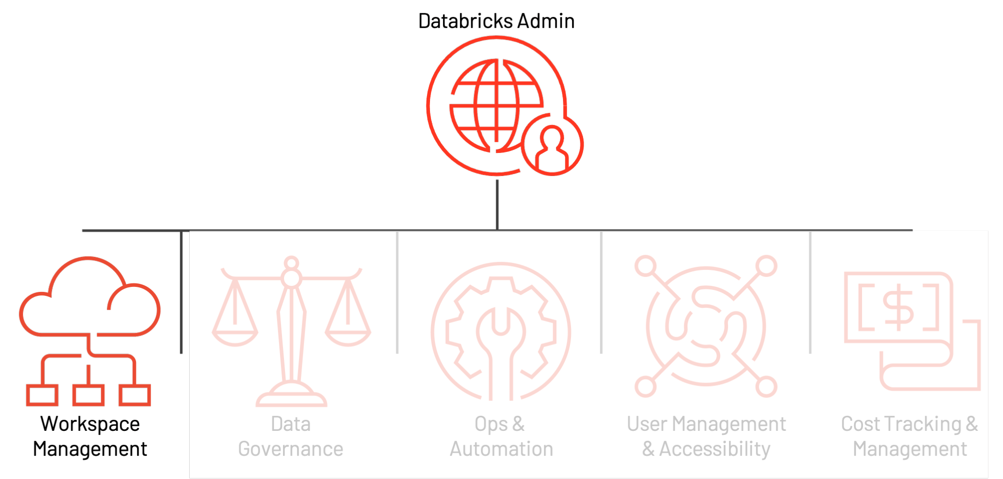
Functional Workspace Organization on Databricks

$
0
0

Introduction

This blog is part one of our Admin Essentials series, where we’ll focus on topics that are important to those managing and maintaining Databricks environments. Keep an eye out for additional blogs on data governance, ops & automation, user management & accessibility, and cost tracking & management in the near future!

In 2020, Databricks began releasing private previews of several platform features known collectively as Enterprise 2.0 (or E2); these features provided the next iteration of the Lakehouse platform, creating the scalability and security to match the power and speed already available on Databricks. When Enterprise 2.0 was made publicly available, one of the most anticipated additions was the ability to create multiple workspaces from a single account. This feature opened new possibilities for collaboration, organizational alignment, and simplification. As we have found since, however, it has also raised a host of questions. Based on our experience across enterprise customers of every size, shape and vertical, this blog will lay out answers and best practices to the most common questions around workspace management within Databricks; at a fundamental level, this boils down to a simple question: exactly when should a new workspace be created? Specifically, we’ll highlight the key strategies for organizing your workspaces, and best practices of each.

Good workspace management is a cornerstone of effective Databricks administration.

Workspace organization basics

Although each cloud provider (AWS, Azure and GCP) has a different underlying architecture, the organization of Databricks workspaces across clouds is similar. The logical top level construct is an E2 master account (AWS) or a subscription object (Azure Databricks/GCP). In AWS, we provision a single E2 account per organization that provides a unified pane of visibility and control to all workspaces. In this way, your admin activity is centralized, with the ability to enable SSO, Audit Logs, and Unity Catalog. Azure has relatively less restriction on creation of top-level subscription objects; however, we still recommend that the number of top-level subscriptions used to create Databricks workspaces be controlled as much as possible. We will refer to the top-level construct as an account throughout this blog, whether it is an AWS E2 account or GCP/Azure subscription.

Within a top-level account, multiple workspaces can be created. The recommended max workspaces per account is between 20 and 50 on Azure, with a hard limit on AWS. This limit arises from the administrative overhead that stems from a growing number of workspaces: managing collaboration, access, and security across hundreds of workspaces can become an extremely difficult task, even with exceptional automation processes. Below, we present a high-level object model of a Databricks account.

high-level object model of a Databricks account.

Enterprises need to create resources in their cloud account to support multi-tenancy requirements. The creation of separate cloud accounts and workspaces for each new use case does have some clear advantages: ease of cost tracking, data and user isolation, and a smaller blast radius in case of security incidents. However, account proliferation brings with it a separate set of complexities – governance, metadata management and collaboration overhead grow along with the number of accounts. The key, of course, is balance. Below, we’ll first go through some general considerations for enterprise workspace organization; then, we’ll go through two common workspace isolation strategies that we see among our customers: LOB-based and product-based. Each has strengths, weaknesses and complexities that we will discuss before giving best practices.

General workspace organization considerations

When designing your workspace strategy, the first thing we often see customers jump to is the macro-level organizational choices; however, there are many lower-level decisions that are just as important! We’ve compiled the most pertinent of these below.

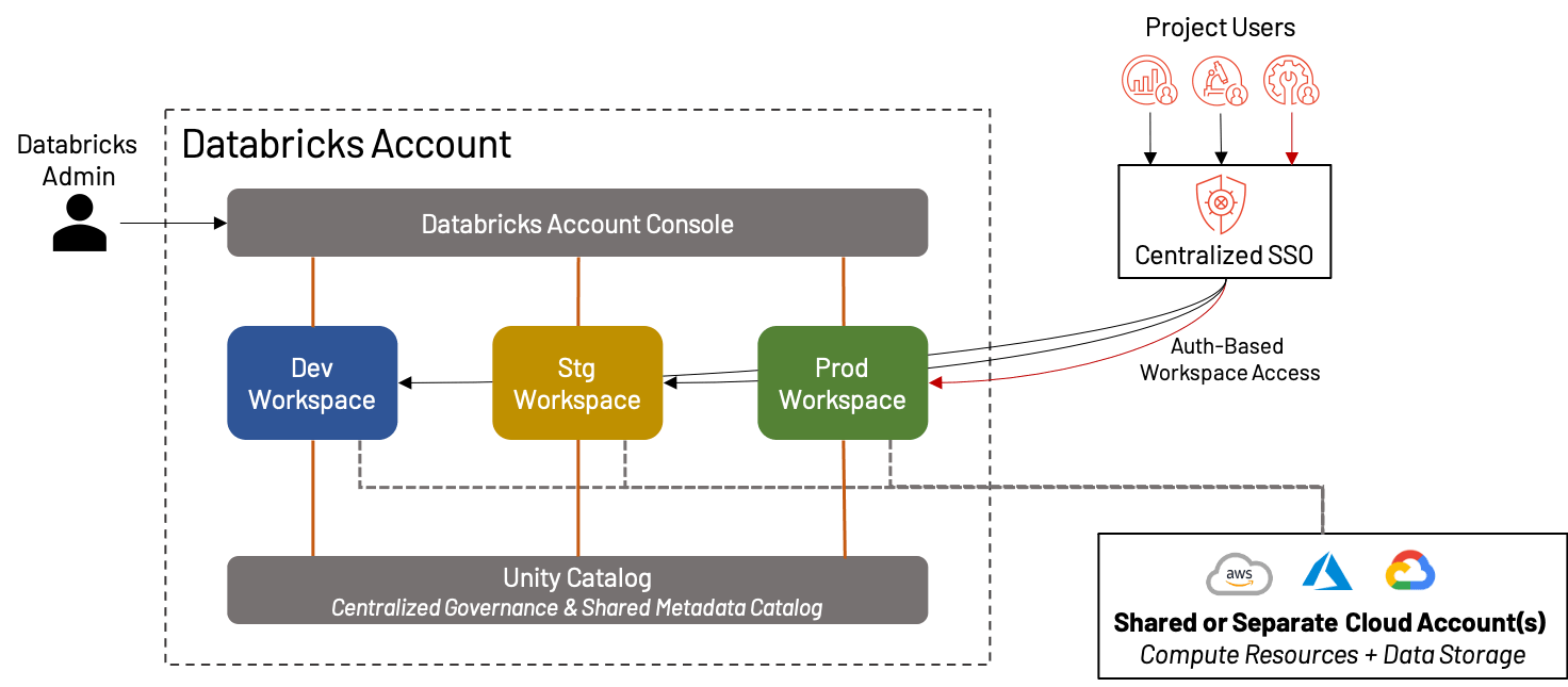
A simple three-workspace approach

Although we spend most of this blog talking about how to split your workspaces for maximum effectiveness, there are a whole class of Databricks customers for whom a single, unified workspace per environment is more than enough! In fact, this has become more and more practical with the rise of features like Repos, Unity Catalog, persona-based landing pages, etc. In such cases, we still recommend the separation of Development, Staging and Production workspaces for validation and QA purposes. This creates an environment ideal for small businesses or teams that value agility over complexity.

Databricks recommends the separation of Development, Staging and Production workspaces for validation and QA purposes.

The benefits and drawbacks of creating a single set of workspaces are:

+ There is no concern of cluttering the workspace internally, mixing assets, or diluting the cost/usage across multiple projects/teams; everything is in the same environment

+ Simplicity of organization means reduced administrative overhead

For larger organizations, a single dev/stg/prd workspace is untenable due to platform limits, clutter, inability to isolate data, and governance concerns

If a single set of workspaces seems like the right approach for you, the following best practices will help keep your Lakehouse operating smoothly:

  • Define a standardized process for pushing code between the various environments; because there is only one set of environments, this may be simpler than with other approaches. Leverage features such as Repos and Secrets and external tools that foster good CI/CD processes to make sure your transitions occur automatically and smoothly.
  • Establish and regularly review Identity Provider groups that are mapped to Databricks assets; because these groups are the primary driver of user authorization in this strategy, it is crucial that they be accurate, and that they map to the appropriate underlying data and compute resources. For example, most users likely do not need access to the production workspace; only a small handful of engineers or admins may have the permissions.
  • Keep an eye on your usage and know the Databricks Resource Limits; if your workspace usage or user count starts to grow, you may need to consider adopting a more involved workspace organization strategy to avoid per-workspace limits. Leverage resource tagging wherever possible in order to track cost and usage metrics.

Leveraging sandbox workspaces

In any of the strategies mentioned throughout this article, a sandbox environment is a good practice to allow users to incubate and develop less formal, but still potentially valuable work. Critically, these sandbox environments need to balance the freedom to explore real data with protection against unintentionally (or intentionally) impacting production workloads. One common best practice for such workspaces is to host them in an entirely separate cloud account; this greatly limits the blast radius of users in the workspace. At the same time, setting up simple guardrails (such as Cluster Policies, limiting the data access to “play” or cleansed datasets, and closing down outbound connectivity where possible) means users can have relative freedom to do (almost) whatever they want to do without needing constant admin supervision. Finally, internal communication is just as important; if users unwittingly build an amazing application in the Sandbox that attracts thousands of users, or expect production-level support for their work in this environment, those administrative savings will evaporate quickly.

Best practices for sandbox workspaces include:

  • Use a separate cloud account that does not contain sensitive or production data.
  • Set up simple guardrails so that users can have relative freedom over the environment without needing admin oversight.
  • Communicate clearly that the sandbox environment is “self-service.”

Data isolation & sensitivity

Sensitive data is growing in prominence among our customers in all verticals; data that was once limited to healthcare providers or credit card processors is now becoming source for understanding patient analysis or customer sentiment, analyzing emerging markets, positioning new products, and almost anything else you can think of. This wealth of data comes with high potential risk, with ever-increasing threats of data breaches; for this reason, keeping sensitive data segregated and protected is important no matter what organizational strategy you choose. Databricks provides several means to protect sensitive data (such as ACLs and secure sharing), and combined with cloud provider tools, can make the Lakehouse you build as low-risk as possible. Some of the best practices around Data Isolation & Sensitivity include:

  • Understand your unique data security needs; this is the most important point. Every business has different data, and your data will drive your governance.
  • Apply policies and controls at both the storage level and at the metastore. S3 policies and ADLS ACLs should always be applied using the principle of least-access. Leverage Unity Catalog to apply an additional layer of control over data access.
  • Separate your sensitive data from non-sensitive data both logically and physically; many customers use entirely separate cloud accounts (and Databricks workspaces) for sensitive and non-sensitive data.

DR and regional backup

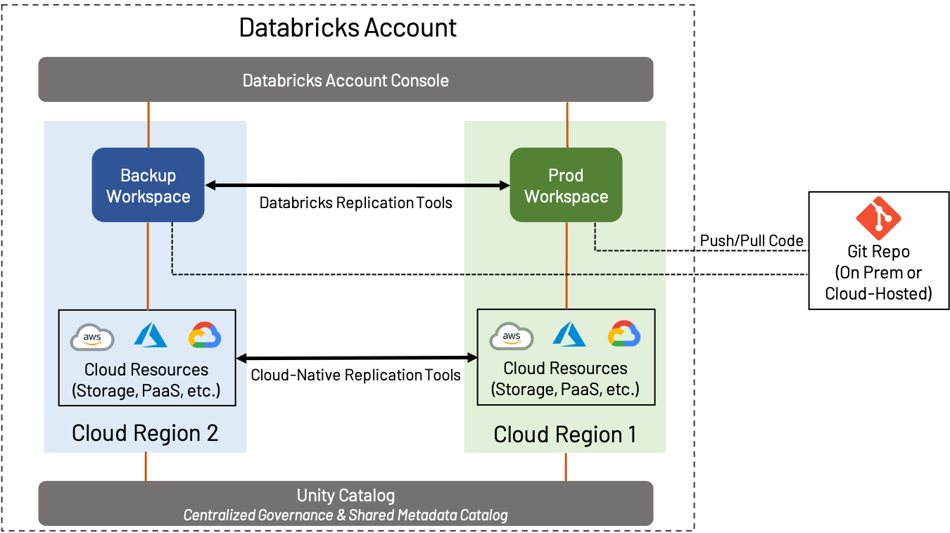
Disaster Recovery (DR) is a broad topic that is important whether you use AWS, Azure or GCP; we won’t cover everything in this blog, but will rather focus on how DR and Regional considerations play into workspace design. In this context, DR implies the creation and maintenance of a workspace in a separate region from the standard Production workspace.

At Databricks, Disaster Recover iimplies the creation and maintenance of a workspace in a separate region from the standard Production workspace.

DR strategy can vary widely depending on the needs of the business. For example, some customers prefer to maintain an active-active configuration, where all assets from one workspace are constantly replicated to a secondary workspace; this provides the maximum amount of redundancy, but also implies complexity and cost (constantly transferring data cross-region and performing object replication and deduplication is a complicated process). On the other hand, some customers prefer to do the minimum necessary to ensure business continuity; a secondary workspace may contain very little until failover occurs, or may be backed up only on an occasional basis. Determining the right level of failover is crucial.

Regardless of what level of DR you choose to implement, we recommend the following:

  • Store code in a Git repository of your choice, either on-prem or in the cloud, and use features such as Repos to sync it to Databricks wherever possible.
  • Whenever possible, use Delta Lake in conjunction with Deep Clone to replicate data; this provides an easy, open-source way to efficiently back up data.
  • Use the cloud-native tools provided by your cloud provider to perform backup of things such as data not stored in Delta Lake, external databases, configurations, etc.
  • Use tools such as Terraform to back up objects such as notebooks, jobs, secrets, clusters, and other workspace objects.

Remember: Databricks is responsible for maintaining regional workspace infrastructure in the Control Plane, but you are responsible for your workspace-specific assets, as well as the cloud infrastructure your production jobs rely upon.

Isolation by line of business (LOB)

We now dive into the actual organization of workspaces in an enterprise context. LOB-based project isolation grows out of the traditional enterprise-centric way of looking at IT resources – it also carries many traditional strengths (and weaknesses) of LOB-centric alignment. As such, for many large businesses, this approach to workspace management will come naturally.

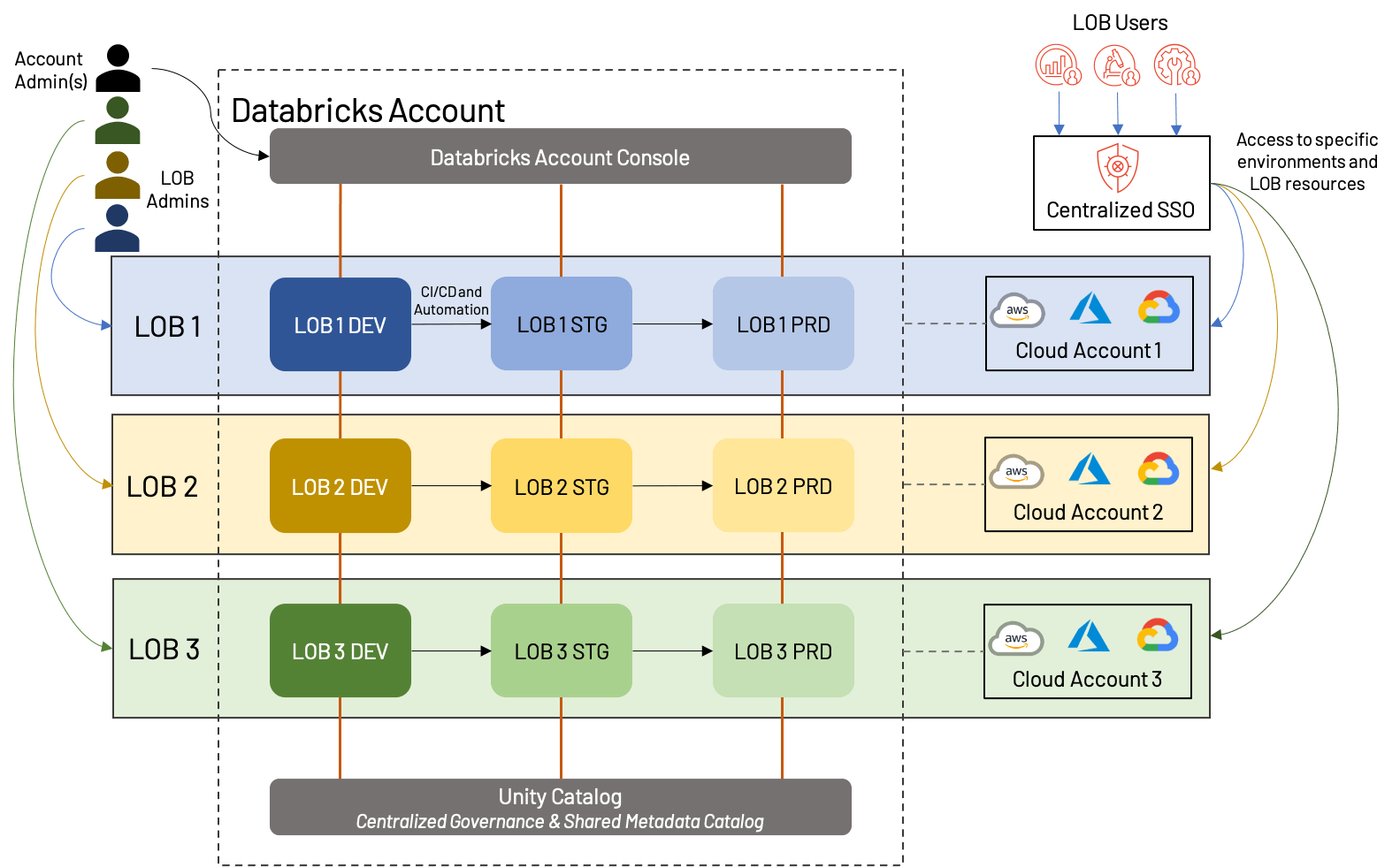
In an LOB-based workspace strategy, each functional unit of a business will receive a set of workspaces; traditionally, this will include development, staging, and production workspaces, although we have seen customers with up to 10 intermediate stages, each potential with their own workspace (not recommended)! Code is written and tested in DEV, then promoted (via CI/CD automation) to STG, and finally lands in PRD, where it runs as a scheduled job until being deprecated. Environment type and independent LOB are the primary reasons to initiate a new workspace in this model; doing so for every use case or data product may be excessive.

One potential way that line of-business-based workspace can be structured.

The above diagram shows one potential way that LOB-based workspace can be structured; in this case, each LOB has a separate cloud account with one workspace in each environment (dev/stg/prd) and also has a dedicated admin. Importantly, all of these workspaces fall under the same Databricks account, and leverage the same Unity Catalog. Some variations would include sharing cloud accounts (and potentially underlying resources such as VPCs and cloud services), using a separate dev/stg/prd cloud account, or creating separate external metastores for each LOB. These are all reasonable approaches that depend heavily on business needs.

Overall, there are a number of benefits, as well as a few drawbacks to the LOB approach:

+Assets for each LOB can be isolated, both from a cloud perspective and from a workspace perspective; this makes for simple reporting/cost analysis, as well as a less cluttered workspace.

+Clear division of users and roles improves the overall governance of the Lakehouse, and reduces overall risk.

+Automation of promotion between environments creates an efficient and low-overhead process.

Up-front planning is required to ensure that cross-LOB processes are standardized, and that the overall Databricks account will not hit platform limits.

Automation and administrative processes require specialists to set up and maintain.

As best practices, we recommend the following to those building LOB-based Lakehouses:

  • Employ a least-privilege access model using fine-grained access control for users and environments; in general, very few users should have production access, and interactions with this environment should be automated and highly controlled. Capture these users and groups in your identity provider and sync them to the Lakehouse.
  • Understand and plan for both cloud provider and Databricks platform limits; these include, for example, the number of workspaces, API rate limiting on ADLS, throttling on Kinesis streams, etc.
  • Use a standardized metastore/catalog with strong access controls wherever possible; this allows for re-use of assets without compromising isolation. Unity Catalog allows for fine-grained controls over tables and workspace assets, which includes objects such as MLflow experiments.
  • Leverage data sharing wherever possible to securely share data between LOBs without needing to duplicate effort.

Data product isolation

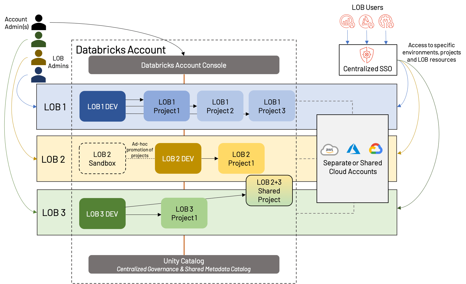
What do we do when LOBs need to collaborate cross-functionally, or when a simple dev/stg/prd model does not fit the use cases of our LOB? We can shed some of the formality of a strict LOB-based Lakehouse structure and embrace a slightly more modern approach; we call this workspace isolation by Data Product. The concept is that instead of isolating strictly by LOB, we isolate instead by top-level projects, giving each a production environment. We also mix in shared development environments to avoid workspace proliferation and make reuse of assets simpler.

Data product isolation: Instead of isolating strictly by LOB, we isolate instead by top-level projects, giving each a production environment.

At first glance, this looks similar to the LOB-based isolation from above, but there are a few important distinctions:

  • A shared dev workspace, with separate workspaces for each top-level project (which means each LOB may have a different number of workspaces overall)
  • The presence of sandbox workspaces, which are specific to an LOB, and offer more freedom and less automation than traditional Dev workspaces
  • Sharing of resources and/or workspaces; this is also possible in LOB-based architectures, but is often complicated by more rigid separation

This approach shares many of the same strengths and weaknesses as LOB-based isolation, but offers more flexibility and emphasizes the value of projects in the modern Lakehouse. More and more, we see this becoming the “gold standard” of workspace organization, corresponding with the movement of technology from primarily a cost-driver to a value generator. As always, business needs may drive slight deviations from this sample architecture, such as dedicated dev/stg/prd for particularly large projects, cross-LOB projects, more or less segregation of cloud resources, etc. Regardless of the exact structure, we suggest the following best practices:

  • Share data and resources whenever possible; although segregation of infrastructure and workspaces is useful for governance and tracking, proliferation of resources quickly becomes a burden. Careful analysis ahead of time will help to identify areas of re-use.
  • Even when not sharing extensively between projects, use a shared metastore such as Unity Catalog, and shared code-bases (via, i.e., Repos) where possible.
  • Use Terraform (or similar tools) to automate the process of creating, managing and deleting workspaces and cloud infrastructure.
  • Provide flexibility to users via sandbox environments, but ensure that these have appropriate guard rails set up to limit cluster sizes, data access, etc.

Summary

To fully leverage all the benefits of the Lakehouse and support future growth and manageability, care should be taken to plan workspace layout. Other associated artifacts that need to be considered during this design include a centralized model registry, codebase, and catalog to aid collaboration without compromising security. To summarize some of the best practices highlighted throughout this article, our key takeaways are listed below:

Best Practice #1: Minimize the number of top-level accounts (both at the cloud provider and Databricks level) where possible, and create a workspace only when separation is necessary for compliance, isolation, or geographical constraints. When in doubt, keep it simple!

Best Practice #2: Decide on an isolation strategy that will provide you long-term flexibility without undue complexity. Be realistic about your needs and implement strict guidelines before beginning to onramp workloads to your Lakehouse; in other words, measure twice, cut once!

Best Practice #3: Automate your cloud processes. This ranges every aspect of your infrastructure (many of which will be covered in following blogs!), including SSO/SCIM, Infrastructure-as-Code with a tool such as Terraform, CI/CD pipelines and Repos, cloud backup, and monitoring (using both cloud-native and third-party tools).

Best Practice #4: Consider establishing a COE team for central governance of an enterprise-wide strategy, where repeatable aspects of a data and machine learning pipeline is templatized and automated so that different data teams can use self-service capabilities with enough guardrails in place. The COE team is often a lightweight but critical hub for data teams and should view itself as an enabler- maintaining documentation, SOPs, how-tos and FAQs to educate other users.

Best Practice #5: The Lakehouse provides a level of governance that the Data Lake does not; take advantage! Assess your compliance and governance needs as one of the first steps of establishing your Lakehouse, and leverage the features that Databricks provides to make sure risk is minimized. This includes audit log delivery, HIPAA and PCI (where applicable), proper exfiltration controls, use of ACLs and user controls, and regular review of all of the above.

We’ll be providing more Admin best practice blogs in the near future, on topics from Data Governance to User Management. In the meantime, reach out to your Databricks account team with questions on workspace management, or if you’d like to learn more about best practices on the Databricks Lakehouse Platform!

--

Try Databricks for free. Get started today.

The post Functional Workspace Organization on Databricks appeared first on Databricks.

Top 5 Databricks Performance Tips

$
0
0

Intro

As solutions architects, we work closely with customers every day to help them get the best performance out of their jobs on Databricks –and we often end up giving the same advice. It’s not uncommon to have a conversation with a customer and get double, triple, or even more performance with just a few tweaks. So what’s the secret? How are we doing this? Here are the top 5 things we see that can make a huge impact on the performance customers get from Databricks.

Here’s a TLDR:

  1. Use larger clusters. It may sound obvious, but this is the number one problem we see. It’s actually not any more expensive to use a large cluster for a workload than it is to use a smaller one. It’s just faster. If there’s anything you should take away from this article, it’s this. Read section 1. Really.
  2. Use Photon, Databricks’ new, super-fast execution engine. Read section 2 to learn more. You won’t regret it.
  3. Clean out your configurations. Configurations carried from one Apache Spark™ version to the next can cause massive problems. Clean up! Read section 3 to learn more.
  4. Use Delta Caching. There’s a good chance you’re not using caching correctly, if at all. See Section 4 to learn more.
  5. Be aware of lazy evaluation. If this doesn’t mean anything to you and you’re writing Spark code, jump to section 5.
  6. Bonus tip! Table design is super important. We’ll go into this in a future blog, but for now, check out the guide on Delta Lake best practices.

1. Give your clusters horsepower!

This is the number one mistake customers make. Many customers create tiny clusters of two workers with four cores each, and it takes forever to do anything. The concern is always the same: they don’t want to spend too much money on larger clusters. Here’s the thing: it’s actually not any more expensive to use a large cluster for a workload than it is to use a smaller one. It’s just faster.

The key is that you’re renting the cluster for the length of the workload. So, if you spin up that two worker cluster and it takes an hour, you’re paying for those workers for the full hour. However, if you spin up a four worker cluster and it takes only half an hour, the cost is actually the same! And that trend continues as long as there’s enough work for the cluster to do.

Here’s a hypothetical scenario illustrating the point:

Number of Workers Cost Per Hour Length of Workload (hours) Cost of Workload
1 $1 2 $2
2 $2 1 $2
4 $4 0.5 $2
8 $8 0.25 $2

Notice that the total cost of the workload stays the same while the real-world time it takes for the job to run drops significantly. So, bump up your Databricks cluster specs and speed up your workloads without spending any more money. It can’t really get any simpler than that.

2. Use Photon

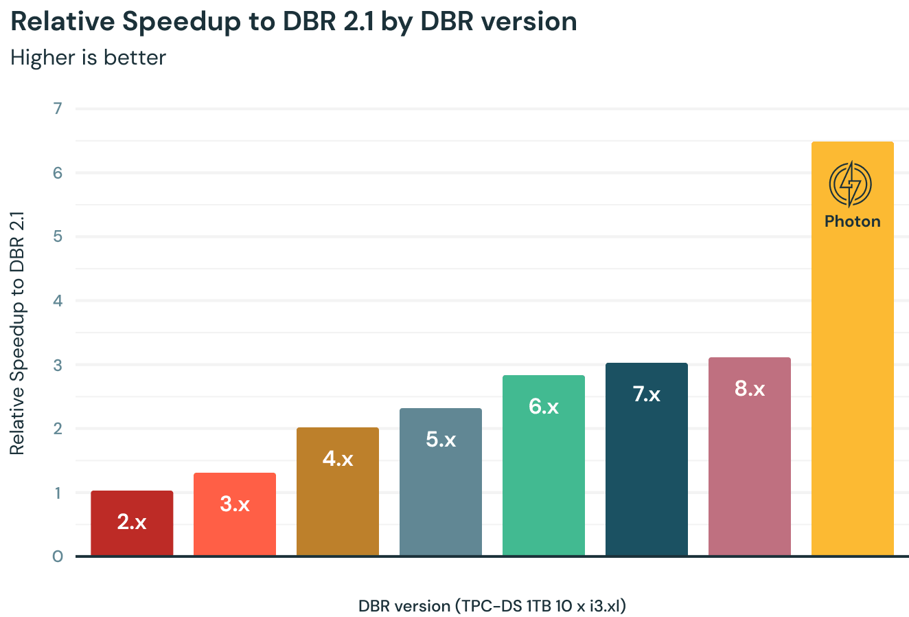
Our colleagues in engineering have rewritten the Spark execution engine in C++ and dubbed it Photon. The results are impressive!

Relative Speedup to Databricks Runtime (DBR) 2.1 by DBR version.

Beyond the obvious improvements due to running the engine in native code, they’ve also made use of CPU-level performance features and better memory management. On top of this, they’ve rewritten the Parquet writer in C++. So this makes writing to Parquet and Delta (based on Parquet) super fast as well!

But let’s also be clear about what Photon is speeding up. It improves computation speed for any built-in functions or operations, as well as writes to Parquet or Delta. So joins? Yep! Aggregations? Sure! ETL? Absolutely! That UDF (user-defined function) you wrote? Sorry, but it won’t help there. The job that’s spending most of its time reading from an ancient on-prem database? Won’t help there either, unfortunately.

The good news is that it helps where it can. So even if part of your job can’t be sped up, it will speed up the other parts. Also, most jobs are written with the native operations and spend a lot of time writing to Delta, and Photon helps a lot there. So give it a try. You may be amazed by the results!

3. Clean out old configurations

You know those Spark configurations you’ve been carrying along from version to version and no one knows what they do anymore? They may not be harmless. We’ve seen jobs go from running for hours down to minutes simply by cleaning out old configurations. There may have been a quirk in a particular version of Spark, a performance tweak that has not aged well, or something pulled off some blog somewhere that never really made sense. At the very least, it’s worth revisiting your Spark configurations if you’re in this situation. Often the default configurations are the best, and they’re only getting better. Your configurations may be holding you back.

4. The Delta Cache is your friend

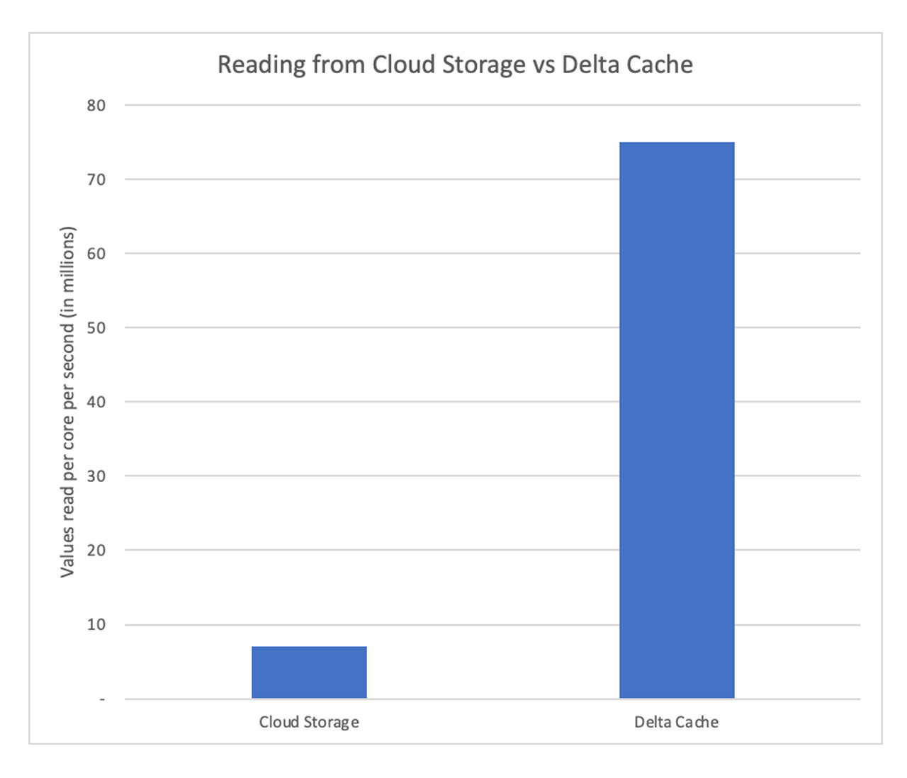
This may seem obvious, but you’d be surprised how many people are not using the Delta Cache, which loads data off of cloud storage (S3, ADLS) and keeps it on the workers’ SSDs for faster access.

If you’re using Databricks SQL Endpoints you’re in luck. Those have caching on by default. In fact, we recommend using CACHE SELECT * FROM table to preload your “hot” tables when you’re starting an endpoint. This will ensure blazing fast speeds for any queries on those tables.

If you’re using regular clusters, be sure to use the i3 series on Amazon Web Services (AWS), L series or E series on Azure Databricks, or n2 in GCP. These will all have fast SSDs and caching enabled by default.

Of course, your mileage may vary. If you’re doing BI, which involves reading the same tables over and over again, caching gives an amazing boost. However, if you’re simply reading a table once and writing out the results as in some ETL jobs, you may not get much benefit. You know your jobs better than anyone. Go forth and conquer.

Reading from cloud storage vs. Delta Cache.

5. Be aware of lazy evaluation

If you’re a data analyst or data scientist only using SQL or doing BI you can skip this section. However, if you’re in data engineering and writing pipelines or doing processing using Databricks / Spark, read on.

When you’re writing Spark code like select, groupBy, filter, etc, you’re really building an execution plan. You’ll notice the code returns almost immediately when you run these functions. That’s because it’s not actually doing any computation. So even if you have petabytes of data it will return in less than a second.

However, once you go to write your results out you’ll notice it takes longer. This is due to lazy evaluation. It’s not until you try to display or write results that your execution plan is actually run.

—--------
# Build an execution plan.
# This returns in less than a second but does no work
df2 = (df
  .join(...)
  .select(...)
  .filter(...)
         )

# Now run the execution plan to get results
df2.display()
—------

However, there is a catch here. Every time you try to display or write out results it runs the execution plan again. Let’s look at the same block of code but extend it and do a few more operations.

—--------
# Build an execution plan.
# This returns in less than a second but does no work
df2 = (df
  .join(...)
  .select(...)
  .filter(...)
         )

# Now run the execution plan to get results
df2.display()

# Unfortunately this will run the plan again, including filtering, joining, etc
df2.display()

# So will this…
df2.count()
—------

The developer of this code may very well be thinking that they’re just printing out results three times, but what they’re really doing is kicking off the same processing three times. Oops. That’s a lot of extra work. This is a very common mistake we run into. So why is there lazy evaluation, and what do we do about it?

In short, processing with lazy evaluation is way faster than without it. Databricks / Spark looks at the full execution plan and finds opportunities for optimization that can reduce processing time by orders of magnitude. So that’s great, but how do we avoid the extra computation? The answer is pretty straightforward: save computed results you will reuse.

Let’s look at the same block of code again, but this time let’s avoid the recomputation:

# Build an execution plan.
# This returns in less than a second but does no work
df2 = (df
  .join(...)
  .select(...)
  .filter(...)
         )

# save it
df2.write.save(path)

# load it back in
df3 = spark.read.load(path)

# now use it
df3.display()

# this is not doing any extra computation anymore.  No joins, filtering, etc.  It’s already done and saved.
df3.display()

# nor is this
df3.count()

This works especially well when Delta Caching is turned on. In short, you benefit greatly from lazy evaluation, but it’s something a lot of customers trip over. So be aware of its existence and save results you reuse in order to avoid unnecessary computation.

Next blog: Design your tables well!

This is an incredibly important topic, but it needs its own blog. Stay tuned. In the meantime, check out this guide on Delta Lake best practices.

--

Try Databricks for free. Get started today.

The post Top 5 Databricks Performance Tips appeared first on Databricks.

Cross-version Testing in MLflow

$
0
0

MLflow is an open source platform that was developed to manage the ML lifecycle, including experimentation, reproducibility, deployment, and a central model registry. It integrates with many popular ML libraries such as scikit-learn, XGBoost, TensorFlow, and PyTorch to support a broad range of use cases. Databricks offers a diverse computing environment with a wide range of pre-installed libraries, including MLflow, that allow customers to develop models without having to worry about dependency management. For example, the table below shows which XGBoost version is pre-installed in different Databricks Runtime for Machine Learning (MLR) environments:

MLR version

Pre-installed XGBoost version

10.3

1.5.1

10.2

1.5.0

10.1

1.4.2

As we can see, different MLR environments provide different library versions. Additionally, users often want to upgrade libraries to try new features. This range of versions poses a significant compatibility challenge and requires a comprehensive testing strategy. Testing MLflow only against one specific version (for instance, only the latest version) is insufficient; we need to test MLflow against a range of ML library versions that users commonly leverage. Another challenge is that ML libraries are constantly evolving and releasing new versions which may contain breaking changes that are incompatible with the integrations MLflow provides (for instance, removal of an API that MLflow relies on for model serialization). We want to detect such breaking changes as early as possible, ideally even before they are shipped in a new version release. To address these challenges, we have implemented cross-version testing.

What is cross-version testing?

Cross-version testing is a testing strategy we implemented to ensure that MLflow is compatible with many versions of widely-used ML libraries (e.g. scikit-learn 1.0 and TensorFlow 2.6.3).

Testing structure

We implemented cross-version testing using GitHub Actions that trigger automatically each day, as well as when a relevant pull request is filed. A test workflow automatically identifies a matrix of versions to test for each of MLflow’s library integrations, creating a separate job for each one. Each of these jobs runs a collection of tests that are relevant to the ML library.

Configuration File

We configure cross-version testing as code using a YAML file that looks like below.

# Integration name
sklearn:
  package_info:
    # Package this integration depends on
    pip_release: "scikit-learn"

    # Command to install the prerelease version of the package
    install_dev: |
      pip install git+https://github.com/scikit-learn/scikit-learn.git

  # Test category. Can be one of ["models", "autologging"]
  # "models" means tests for model serialization and serving
  # "autologging" means tests for autologging
  autologging:
    # Additional requirements to run tests
    # `>= 24.0: ["matplotlib"]` means "Install matplotlib
    # if scikit-learn version is >= 0.24.0"
    requirements:
      ">= 0.24.0": ["matplotlib"]

    # Versions that should not be supported due to unacceptable issues
    unsupported: ["0.22.1"]

    # Minimum supported version
    minimum: "0.20.3"

    # Maximum supported version
    maximum: "1.0.2"

    # Command to run tests
    run: |
      pytest tests/sklearn/autologging

xgboost:
  ...

One of the outcomes of cross-version testing is that MLflow can clearly document which ML library versions it supports and warn users when an installed library version is unsupported. For example, the documentation for the mlflow.sklearn.autolog API provides a range of compatible scikit-learn versions:

Refer to this documentation of the mlflow.sklearn.autolog API for further reading.

Next, let’s take a look at how the unsupported version warning feature works. In the Python script below, we patch sklearn.__version__ with 0.20.2, which is older than the minimum supported version 0.20.3 to demonstrate the feature, and then call mlflow.sklearn.autolog

from unittest import mock
import mlflow

# Assume scikit-learn 0.20.2 is installed
with mock.patch("sklearn.__version__", "0.20.2"):
    mlflow.sklearn.autolog()

The script above prints out the following message to warn the user that the unsupported version of scikit-learn (0.20.2) is being used and autologging may not work properly:

2022/01/21 16:05:50 WARNING mlflow.utils.autologging_utils: You are using an unsupported version of sklearn. If you encounter errors during autologging, try upgrading / downgrading sklearn to a supported version, or try upgrading MLflow.

Running tests

Now that we have a testing structure, let’s run the tests. To start, we created a GitHub Actions workflow that constructs a testing matrix from the configuration file and runs each item in the matrix as a separate job in parallel. An example of the GitHub Actions workflow summary for scikit-learn cross-version testing is shown below. Based on the configuration, we have a minimum version “0.20.3”, which is shown at the top. We populate all versions that exist between that minimum version and the maximum version “1.0.2”. At the bottom, you can see the addition of one final test: the “dev” version, which represents a prerelease version of scikit-learn installed from the main development branch in scikit-learn/scikit-learn via the command specified in the install_dev field. We’ll explain the aim of this prerelease version testing in the “Testing the future” section later.

MLflow GitHub Actions workflow that constructs a testing matrix from the configuration file and runs each item in the matrix as a separate job in parallel.

Which versions to test

To limit the number of GitHub Actions runs, we only test the latest micro version in each minor version. For instance, if “1.0.0”, “1.0.1”, and “1.0.2” are available, we only test “1.0.2”. The reasoning behind this approach is that most people don’t explicitly install an old minor version of a major release, and the latest minor version of a major version is typically the most bug-free. The table below shows which versions we test for scikit-learn.

scikit-learn version

Tested

0.20.3

0.20.4

0.21.0


0.21.1


0.21.2


0.21.3

0.22


0.22.1


0.22.2


0.22.2.post1

0.23.0


0.23.1


0.23.2

0.24.0


0.24.1


0.24.2

1.0


1.0.1


1.0.2

dev

When to trigger cross-version testing

There are two events that trigger cross-version testing:

  1. When a relevant pull request is filed. For instance, if we file a PR that updates files under the mlflow/sklearn directory, the cross-version testing workflow triggers jobs for scikit-learn to guarantee that code changes in the PR are compatible with all supported scikit-learn versions.
  2. A daily cron job where we run all cross-version testing jobs including ones for prerelease versions. We check the status of this cron job every working day to catch issues as early as possible.

Testing the future

In cross-version testing, we run daily tests against both publicly available versions and prerelease versions installed from on the main development branch for all dependent libraries that are used by MLflow. This allows us to predict what will happen to MLflow in the future.

Let’s take a look at a real situation that the MLflow maintainers recently handled:

  • On 2021/12/26, LightGBM removed several deprecated function arguments in microsoft/LightGBM#4908. This change broke MLflow’s autologging integration for LightGBM.
  • On 2021/12/27, we found one of cross-version test runs for LightGBM failed and identified microsoft/LightGBM#4908 as the root cause.
  • Real-world example of MLflow cross-version testing.

  • On 2021/12/28, we filed a PR to fix this issue: mlflow/mlflow#5206
  • On 2021/12/31, we merged the PR.
  • On 2022/01/08, LightGBM 3.3.2 was released, containing the breaking change.
  |
  ├─ 2021/12/26 microsoft/LightGBM#4908 (breaking change) was merged.
  ├─ 2021/12/27 Found LightGBM test failure
  ├─ 2021/12/28 Filed mlflow/mlflow#5206
  |
  ├─ 2021/12/31 Merged mlflow/mlflow#5206.
  |
  |
  ├─ 2022/01/08 LightGBM 3.3.2 release
  |
  |
  ├─ 2022/01/17 MLflow 1.23.0 release
  |
  v
 time

Thanks to prerelease version testing, we were able to discover the breaking change the day after, it was merged and quickly apply a patch for it even before the LightGBM 3.3.2 release. This proactive work, handled ahead of time and on a less-urgent schedule, allowed us to be prepared for their new release and avoid breaking changes or regressions.

If we didn’t perform prerelease version testing, we would have only discovered the breaking change after the LightGBM 3.3.2 release, which could have resulted in a broken user experience depending on the LightGBM release date. For example, consider the problematic scenario below where LightGBM was released after MLflow without prerelease version testing. Users running LightGBM 3.3.2 and MLflow 1.23.0 would have encountered bugs.

  |
  ├─ 2021/12/26 microsoft/LightGBM #4908 (breaking change) was merged.
  |
  |
  ├─ 2022/01/17 MLflow 1.23.0 release                         
  |
  ├─ 2022/01/20 (hypothetical) LightGBM 3.3.2 release
  ├─ 2022/01/21 Users running LightGBM 3.3.2 and MLflow 1.23.0
  |             would have encountered bugs.
  |  
  v
 time

Conclusion

In this blog post, we covered:

  • Why we implemented cross-version testing.
  • How we configure and run cross-version testing.
  • How we enhance the MLflow user experience and documentation using the cross-version testing outcomes.

Check out this README file for further reading on the implementation of cross-version testing. We hope this blog post will help other open-source projects that provide integrations for many ML libraries.

--

Try Databricks for free. Get started today.

The post Cross-version Testing in MLflow appeared first on Databricks.

Riding the AI Wave

$
0
0

“…incorporating machine learning into a company’s application development is difficult…”

It’s been almost a decade since Marc Andreesen hailed that software was eating the world and, in tune with that, many enterprises have now embraced agile software engineering and turned it into a core competency within their organization. Once ‘slow’ enterprises have managed to introduce agile development teams successfully, with those teams decoupling themselves from the complexity of operational data stores, legacy systems and third-party data products by interacting ‘as-a-service’ via APIs or event-based interfaces. These teams can instead focus on the delivery of solutions that support business requirements and outcomes seemingly having overcome their data challenges.

Of course, little stays constant in the world of technology. The impact of cloud computing, huge volumes and new types of data, and more than a decade of close collaboration between research and business has created a new wave. Let’s call this new wave the AI wave.

Artificial intelligence (AI) gives you the opportunity to go beyond purely automating how people work. Instead, data can be exploited to automate predictions, classifications and actions for more effective, timely decision making – transforming aspects of your business such as responsive customer experience. Machine learning (ML) goes further to train off-the-shelf models to meet requirements that have proven too complex for coding alone to address.

But here’s the rub: incorporating ML into a company’s application development is difficult. ML right now is a more complex activity than traditional coding. Matei Zaharia, Databricks co-founder and Chief Technologist, proposed three reasons for that. First, the functionality of a software component reliant on ML isn’t just built using coded logic, as is the case in most software development today. It depends on a combination of logic, training data and tuning. Second, its focus isn’t in representing some correct functional specification, but on optimizing the accuracy of its output and maintaining that accuracy once deployed. And finally, the frameworks, model architectures and libraries a ML engineer relies on typically evolve quickly and are subject to change.

Each of these three points bring their own challenges, but within this article I want to focus on the first point, which highlights the fact that data is required within the engineering process itself. Until now, application development teams have been more concerned with how to connect to data at test or runtime, and they solved problems associated with that by building APIs, as described earlier. But those same APIs don’t help a team exploiting data during development time. So, how do your projects harness less code and more training data in their development cycle?

The answer is closer collaboration between the data management organization and application development teams. There is currently much discussion reflecting this, perhaps most prominently centered on the idea of data mesh (Dehghani 2019). My own experience over the last few decades has flip-flopped between the application and data worlds, and drawing from that experience, I position seven practices that you should consider when aligning teams across the divide.

  1. Use a design first approach to identify the most important data products to build

    Successful digital transformations are commonly led by transforming customer engagement. Design first – looking at the world through your customer’s eyes – has been informing application development teams for some time. For example, frameworks such as ‘Jobs to be Done’ introduced by Clayton Christensen et al focuses design on what a customer is ultimately trying to accomplish. Such frameworks help development teams identify, prioritize and then build features based on the impact they provide to their customers achieving their desired goals.

    Likewise, the same design first approach can identify which data products should be built, allowing an organization to challenge itself on how AI can have the most customer impact. Asking questions like ‘What decisions need to be made to support the customer’s jobs-to-be-done?’ can help identify which data and predictions are needed to support those decisions, and most importantly, the data products required, such as classification or regression ml models.

    It follows that both the backlogs of application features and data products can derive from the same design first exercise, which should include data scientist and data architect participation alongside the usual business stakeholder and application architect participants. Following the exercise, this wider set of personas must collaborate on an ongoing basis to ensure dependencies across features and data product backlogs are managed effectively over time. That leads us neatly to the next practice.

  2. Organize effectively across data and application teams

    We’ve just seen how closer collaboration between data teams and application teams can inform the data science backlog (research goals) and associated ML model development carried out by data scientists. Once a goal has been set, it’s important to resist progressing the work independently. The book Executive Data Science by Caffo and colleagues highlights two common organizational approaches – embedded and dedicated – that inform the team structures adopted to address common difficulties in collaboration. On one hand, in the dedicated model, data roles such as data scientists are permanent members of a business area application team (a cross functional team). On the other hand, in the embedded model, those data roles are members of a centralized data organization and are then embedded in the business application area.

    Data & AI COE in a federated organization

    Figure 1 COEs in a federated organization

    In a larger organization with multiple lines of business, where potentially many agile development streams require ML model development, isolating that development into a dedicated center of excellence (COE) is an attractive option. Our Shell case study describes how a COE can drive successful adoption of AI, and a COE combines well with the embedded model (as illustrated in Figure 1). In that case, COE members are tasked with delivering the AI backlog. However, to support urgency, understanding and collaboration, some of the team members are assigned to work directly within the application development teams. Ultimately, the best operating model will be dependent on the maturity of the company, with early adopters maintaining more skills in the ‘hub’ and mature adopters with more skills in the ‘spokes.’

  3. Support local data science by moving ownership and visibility of data products to decentralized business focused teams

    Another important organizational aspect to consider is data ownership. Where risks around data privacy, consent and usage exist, it makes sense that accountability for the ownership and managing of those risks is accepted within the area of the business that best understands the nature of the data and its relevance. AI introduces new data risks, such as bias, explainability and ensuring ethical decisions. This creates a pressure to build siloed data management solutions where a sense of control and total ownership is established, leading to siloes that resist collaboration. Those barriers inevitably lead to lower data quality across the enterprise, for example affecting the accuracy of customer data through siloed datasets being developed with overlapping, incomplete or inconsistent attributes. Then that lower quality is perpetuated into models trained by that data.

    Figure 2 Local ownership of data products in a data mesh

    The concept of a data mesh has gained traction as an approach for local business areas to maintain ownership of data products while avoiding the pitfalls of adopting a siloed approach. In a data mesh, datasets can be owned locally, as pictured in Figure 2. Mechanisms can then be put in place allowing them to be shared in the wider organization in a controlled way, and within the risk parameters determined by the data product’s owner. Lakehouse provides a data platform architecture that naturally supports a data mesh approach. Here, an organization’s data supports multiple data product types – such as models, datasets, BI dashboards and pipelines – on a unified data platform that enables independence of local areas across the business. With lakehouse, teams create their own curated datasets using the storage and compute they can control. Those products are then registered in a catalog allowing easy discovery and self-service consumption, but with appropriate security controls to open access only to other permitted groups in the wider enterprise.

  4. Minimize time required to move from idea to solution with consistent DataOps

    Once the backlog is defined and teams are organized, we need to address how data products, such as the models appearing in the backlog, are developed … and how that can be built quickly. Data ingestion and preparation are the biggest efforts of model development, and effective DataOps is the key to minimize them. For example, Starbucks built an analytics framework, BrewKit, based on Azure Databricks, that focuses on enabling any of their teams, regardless of size or engineering maturity, to build pipelines that tap into the best practices already in place across the company. The goal of that framework is to increase their overall data processing efficiency; they’ve built more than 1000 data pipelines with up to 50-100x faster data processing. One of the framework’s key elements is a set of templates that local teams can use as the starting point to solve specific data problems. Since the templates rely on Delta Lake for storage, solutions built on the templates don’t have to solve a whole set of concerns when working with data on cloud object storage, such as pipeline reliability and performance.

    There is another critical aspect of effective DataOps. As the name suggests, DataOps has a close relationship with DevOps, the success of which relies heavily on automation. An earlier blog, Productionize and Automate your Data Platform at Scale, provides an excellent guide on that aspect.

    It’s common to need whole chain of transformations to take raw data and turn it into a format suitable for model development. In addition to Starbucks,, we’ve seen many customers develop similar frameworks to accelerate their time to build data pipelines. With this in mind, Databricks launched Delta Live Tables, which simplifies creating reliable production data pipelines and solves a host of problems associated with their development and operation

  5. Be realistic about sprints for model development versus coding

    It’s an attractive idea that all practices from the application development world can translate easily to building data solutions. However, as pointed out by Matei Zaharia, traditional coding and model development have different goals. On one hand, coding’s goal is the implementation of some set of known features to meet a clearly defined functional specification. On the other hand, the goal of model development is to optimize the accuracy of a model’s output, such as a prediction or classification, and then maintaining that accuracy over time. With application coding, if you are working on fortnightly sprints, it’s likely you can break down functionality into smaller units with a goal to launch a minimal viable product and then incrementally, sprint by sprint, add new features to the solution. However, what does ‘breaking down’ mean for model development? Ultimately, the compromise would require a less optimized, and correspondingly, less accurate model. A minimal viable model here means a less optimal model, and there is only so low in accuracy you can go before a sub optimal model doesn’t provide sufficient value in a solution, or drives your customers crazy. So, the reality here is some model development will not fit neatly into the sprints associated with application development.

    So, what does that dose of realism mean? While there might be an impedance mismatch between the clock-speed of coding and model development, you can at least make the ML lifecycle and data scientist or ML engineers as effective and efficient as possible, thereby reducing the time to arriving at a first version of the model with acceptable accuracy – or deciding acceptable accuracy won’t be possible and bailing out. Let’s see how that can be done next.

  6. Adopt consistent MLOps and automation to make data scientists zing

    Efficient DataOps described in practice #4 provides large benefits for developing ML models – the data collection, data preparation and data exploration required, as DataOps optimizations will expedite prerequisites for modeling. We discuss this further in the blog The Need for Data-centric ML Platforms, which describes the role of a lakehouse approach to underpin ML. In addition, there are very specific steps that are the focus of their own unique practices and tooling in ML development. Finally, once a model is developed, it needs to be deployed using DevOps-inspired best practices. All these moving parts are captured in MLOps, which focuses on optimizing every step of developing, deploying and monitoring models throughout the ML model lifecycle, as illustrated on the Databricks platform in figure 3.

    Figure 3 The component parts of MLOps with Databricks

    It is now commonplace in the application development world to use consistent development methods and frameworks alongside automating CI/CD pipelines to accelerate the delivery of new features. In the last 2 to 3 years, similar practices have started to emerge in data organizations that support more effective MLops. A widely-adopted component contributing to that growing maturity is MLflow, the open source framework for managing the ML lifecycle, which Databricks provides as a managed service. Databricks customers such as H&M have industrialized ML in their organizations building more models, faster by putting MLflow at the heart of their model operations. Automation opportunities go beyond tracking and model pipelines. AutoML techniques can further boost data scientists’ productivity by automating large amounts of the experimentation involved in developing the best model for a particular use case.

  7. To truly succeed with AI at scale, it’s not just data teams – application development organizations must change too

    Much of the change related to these seven points will most obviously impact data organizations. That’s not to say that application development teams don’t have to make changes too. Certainly, all aspects related to collaboration rely on commitment from both sides. But with the emergence of lakehouse, DataOps, MLOps and a quickly-evolving ecosystem of tools and methods to support data and AI practices, it is easy to recognise the need for change in the data organization. Such cues might not immediately lead to change though. Education and evangelisation play a crucial role in motivating teams how to realign and collaborate differently. To permeate the culture of a whole organization, a data literacy and skills programme is required and should be tailored to the needs of each enterprise audience including application development teams.

    Hand in hand with promoting greater data literacy, application development practices and tools must be re-examined as well. For example, ethical issues can impact application coders’ common practices, such as reusing APIs as building blocks for features. Consider the capability ‘assess credit worthiness’, whose implementation is built with ML. If the model endpoint providing the API’s implementation was trained with data from an area of a bank that deals with high wealth individuals, that model might have significant bias if reused in another area of the bank dealing with lower income clients. In this case, there should be defined processes to ensure application developers or architects scrutinize the context and training data lineage of the model behind the API. That can uncover any issues before making the decision to reuse, and discovery tools must provide information on API context and data lineage to support that consideration.

In summary, only when application development teams and data teams work seamlessly together will AI become pervasive in organizations. While commonly those two worlds are siloed, increasingly organizations are piecing together the puzzle of how to set the conditions for effective collaboration. The seven practices outlined here capture best practices and technology choices adopted in Databricks’ customers to achieve that alignment. With these in place, organizations can ride the AI wave, changing our world from one eaten by software to a world instead where machine learning is eating software.

Find out more about how your organization can ride the AI wave by checking out the Enabling Data and AI at Scale strategy guide, which describes the best practices building data-driven organizations. Also, catch up with the 2021 Gartner Magic Quadrants (MQs) where Databricks is the only cloud-native vendor to be named a leader in both the Cloud Database Management Systems and the Data Science and Machine Learning Platforms MQs.

--

Try Databricks for free. Get started today.

The post Riding the AI Wave appeared first on Databricks.

Dominate Your Daily Wordle With Lakehouse

$
0
0

Since it launched late last year, Wordle has become a daily highlight for people around the world. So much, that the New York Times recently acquired the puzzle game to add to its growing portfolio. At Databricks, there are few things that we enjoy more than finding new, innovative ways to leverage our Lakehouse platform. So, we thought: why not use it to increase our competitive edge with Wordle?

This blog post will walk through how we executed this use case by analyzing Wordle data to identify the most frequent letters used on the platform. We made it easy for you to use our results to identify additional words that can help you with your daily Wordle!

What is Wordle?

For those unfamiliar, Wordle is a simple word-solving game that comes out daily. At a high level, you have 6 attempts to guess a 5-letter word; after submitting each guess, the player is given clues as to how many letters were guessed correctly. You can view the full instructions (and play!) here.

Our Approach

For this use case, we wanted to answer the question: What are the most optimal words to start with when playing Wordle?

For our data set, we used Wordle’s library of 5 letter words. Using the Databricks Lakehouse Platform, we were able to ingest and cleanse this library, execute two approaches for identifying “optimal” starting words, and extract insights from visualizations to identify these two words. Lakehouse was an ideal choice for this use case since it provides a unified platform that enables end-to-end analytics (data ingestion -> data analysis -> business intelligence); using the Databricks notebook environment, we were able to easily organize our analysis into a defined process.

Data Ingestion, Transformation, and Analysis Process

First, we extracted Wordle’s library of accepted 5 letter words from their website’s page source as a CSV. This library included 12,972 words ranging from “aahed” to “zymic.”

To accelerate the ingestion, transformation, and analytics of the Wordle library, we used the Databricks notebook environment, which allows us to seamlessly use multiple programming languages (SQL, Python, Scala, R), whichever the user is most comfortable with, to define a process for systematically designing and executing the analysis. By using this environment, we were able to collaboratively iterate through the process using the same notebook without having to worry about version control. This simplified the overall process of getting to the optimal starting words.

Using the Databricks notebook environment provided by the Lakehouse, we simply ingested data from a CSV file and loaded it into a Delta table named “wordle.” This raw table we refer to as our “bronze” data table, as per our medallion architecture. The bronze layer contains our raw ingestion and history data. The silver layer contains our transformed (e.g., filtered, cleansed, augmented) data. The gold layer contains the business level aggregated data, ready for insight analysis.

from pyspark.sql.types import StructType, StructField, StringType

schema = StructType([
    StructField("word", StringType(), True)])

df= spark.read.csv("/FileStore/Wordlev2-1.csv", header = "false", schema = schema)

df.write.saveAsTable("wordle")

We identified that the ingestion required data cleansing before being able to perform analytics. For example, “false” was ingested as “FALSE” due to the format in which data was saved, limiting our ability to do character lookups (without additional logic) as “f” is equivalent to “F.” Since the Databricks notebook environment supports multiple programming languages, we used SQL to identify the data quality issues and cleanse this data. We loaded this data into a “silver” table called Wordle_Cleansed.

We then calculated the frequency of each letter across the library of words in Wordle_Cleansed and saved the results in a “gold” Delta table called Word_Count.

Additionally, we calculated the frequency of each letter at each letter position (p_1, p_2, p_3, p_4, p_5) across the library of words and saved the results in “gold” Delta tables for each position (e.g., Word_Count_p1). Finally, we analyzed Word_Count results and each position table to determine scenarios of optimal words. Now let’s dive into our findings.

Outcome: Overall Letter Count

Below are the top 10 letters based on letter frequency in Wordle’s 5 letter accepted word library. After analyzing these letters, we determined that the optimal starting word is “soare,” or young hawk. You can also use the graph to determine other high-value words:

Top 10 Letter Frequency

Outcome: Letter Count by Position

Below are the top letters based on letter frequency and position in Wordle’s accepted word library. After analyzing these distributions, there are a number of different options for “optimal” starting words using this approach. For example, “cares” is a great option. “S” is the most common letter both at position 1 (P1) and at P5. Since it is twice as frequent at P5, we slot it there.

“C” is the next most frequent letter in P1, so we slot it there, giving us “C _ _ _ S.” “A” is the most frequent letter in P2 and P3, but more frequent in P2, so we slot it there. In P3, the second most frequent letter is “R”, so we now have “C A R _ S”. To finish off the word, we look at P4 where “E” is the most frequent letter. As a result, using this approach the “optimal” starting word is “cares.”

Position 1

Position 2

Position 3

Position 4

Position 5

Conclusion

Of course, “optimal” is just one strategic aspect when playing Wordle – so this definitely takes the “puzzle” aspect out of the game. And what’s optimal now will likely evolve over time! That’s why we encourage you to try this use case yourself.

New to Lakehouse? Check out this blog post from our co-founders for an overview of the architecture and how it can be leveraged across data teams.

--

Try Databricks for free. Get started today.

The post Dominate Your Daily Wordle With Lakehouse appeared first on Databricks.

How to Speed Up Data Flow Between Databricks and SAS

$
0
0

This is a collaborative post between Databricks and T1A. We thank Oleg Mikhov, Solutions Architect at T1A, for his contributions.

 
This is the first post in a series of blogs on the best practices of bringing together Databricks Lakehouse Platform and SAS. A previous Databricks blog post introduced Databricks and PySpark to SAS developers. In this post, we discuss ways for exchanging data between SAS and Databricks Lakehouse Platform and ways to speed up the data flow. In future posts, we will explore building efficient data and analytics pipelines involving both technologies.

Data-driven organizations are rapidly adopting the Lakehouse platform to keep up with the constantly growing business demands. Lakehouse platform has become a new norm for organizations wanting to build data platforms and architecture. The modernization entails moving data, applications, or other business elements to the cloud. However, the transition to the cloud is a gradual process and it is business-critical to continue leveraging legacy investments for as long as possible. With that in mind, many companies tend to have multiple data and analytics platforms, where the platforms coexist and complement each other.

One of the combinations we see is the use of SAS with the Databricks Lakehouse. There are many benefits of enabling the two platforms to efficiently work together, such as:

  • Greater and scalable data storage capabilities of cloud platforms
  • Greater computing capacity using technologies, such as Apache Spark™, natively built with parallel processing capabilities
  • Achieve greater compliance with data governance and management using Delta Lake
  • Lower the cost of data analytics infrastructure with simplified architectures

Some common data science and data analysis use cases and reasons observed are:

  1. SAS practitioners leverage SAS for its core statistical packages to develop advanced analytics output that meets regulatory requirements while they use Databricks Lakehouse for data management, ELT types of processing, and data governance
  2. Machine learning models developed in SAS are scored on massive amounts of data using parallel processing architecture of Apache Spark engine in the Lakehouse platform
  3. SAS data analysts gain faster access to large amounts of data in the Lakehouse Platform for ad-hoc analysis and reporting using Databricks SQL endpoints and high bandwidth connectors
  4. Ease cloud modernization and migration journey by establishing a hybrid workstream involving both cloud architecture and on-prem SAS platform

However, a key challenge of this coexistence is how the data is performantly shared between the two platforms. In this blog, we share best practices implemented by T1A for their customers and benchmark results comparing different methods of moving data between Databricks and SAS.

Scenarios

The most popular use case is a SAS developer trying to access data in the lakehouse. The analytics pipelines involving both technologies require data flow in both directions: data moved from Databricks to SAS and data moved from SAS to Databricks.

  1. Access Delta Lake from SAS: A SAS user wants to access big data in Delta Lake using the SAS programming language.
  2. Access SAS datasets from Databricks: A Databricks user wants to access SAS datasets, generally the sas7bdat datasets as a DataFrame to process in Databricks pipelines or store in Delta Lake for enterprise-wide access.

In our benchmark tests, we used the following environment setup:

  1. Microsoft Azure as the cloud platform
  2. SAS 9.4M7 on Azure (single node Standard D8s v3 VM)
  3. Databricks runtime 9.0, Apache Spark 3.1.2 (2 nodes Standard DS4v2 cluster)

Figure 1 shows the conceptual architecture diagram with the components discussed. Databricks Lakehouse sits on Azure Data Lake storage with Delta Lake medallion architecture. SAS 9.4 installed on Azure VM connects to Databricks Lakehouse to read/write data using connection options discussed in the following sections.

SAS and Databricks conceptual architecture diagram on Azure

Figure 1 SAS and Databricks conceptual architecture diagram on Azure

The diagram above shows a conceptual architecture of Databricks deployed on Azure. The architecture will be similar on other cloud platforms. In this blog, we only discuss the integration with the SAS 9.4 platform. In a later blog post, we will extend this discussion to access lakehouse data from SAS Viya.

Access Delta Lake from SAS

Imagine that we have a Delta Lake table that needs to be processed in a SAS program. We want the best performance when accessing this table, while also avoiding any possible issues with data integrity or data types compatibility. There are different ways to achieve data integrity and compatibility. Below we discuss a few methods and compare them on ease of use and performance.

In our testing, we used the eCommerce behavior dataset (5.67GB, 9 columns, ~ 42 mill records) from Kaggle.
Data Source Credit: eCommerce behavior data from multi category store and REES46 Marketing Platform.

Tested methods

1. Using SAS/ACCESS Interface connectors
Traditionally, SAS users leverage SAS/ACCESS software to connect to external data sources. You can either use a SAS LIBNAME statement pointing to the Databricks cluster or use the SQL pass-through facility. At present for SAS 9.4, there are three connection options available.

  1. SAS/ACCESS Interface to ODBC
  2. SAS/ACCESS Interface to JDBC
  3. SAS/ACCESS Interface to Spark

SAS/ACCESS Interface to Spark has been recently loaded with capabilities with exclusive support to Databricks clusters. See this video for a short demonstration. The video mentions SAS Viya but the same is applicable to SAS 9.4.

Code samples on how to use these connectors can be found in this git repository: T1A Git – SAS Libraries Examples.

2. Using saspy package
The open-source library, saspy, from SAS Institute allows Databricks Notebook users to run SAS statements from a Python cell in the notebook to execute code in the SAS server, as well as to import and export data from SAS datasets to Pandas DataFrame.

Since the focus of this section is accessing lakehouse data by a SAS programmer using SAS programming, this method was wrapped in a SAS macro program similar to the purpose-built integration method discussed next.

To achieve better performance with this package, we tested the configuration with a defined char_length option (details available here). With this option, we can define lengths for character fields in the dataset. In our tests using this option brought an additional 15% increase in performance. For the transport layer between environments, we used the saspy configuration with an SSH connection to the SAS server.

3. Using a purpose-built integration
Although the two methods mentioned above have their upsides, the performance can be improved further by addressing some shortcomings, discussed in the next section (Test Results), of the previous methods. With that in mind, we developed a SAS macro-based integration utility with a prime focus on performance and usability for SAS users. The SAS macro can be easily integrated into existing SAS code without any knowledge about Databricks platform, Apache Spark or Python.

The macro orchestrates a multistep process using Databricks API:

  1. Instruct the Databricks cluster to query and extract data per the provided SQL query and cache the results in DBFS, relying on its Spark SQL distributed processing capabilities.
  2. Compress and securely transfer the dataset to the SAS server (CSV in GZIP) over SSH
  3. Unpack and import data into SAS to make it available to the user in the SAS library. At this step, leverage column metadata from Databricks data catalog (column types, lengths, and formats) for consistent, correct and efficient data presentation in SAS

Note that for variable-length data types, the integration supports different configuration options, depending on what best fits the user requirements such as,

  • need for using a configurable default value
  • profiling to 10,000 rows (+ add headroom) to identify the largest value
  • profiling the entire column in the dataset to identify the largest value

A simplified version of the code is available here T1A Git – SAS DBR Custom Integration.

The end-user usage of this SAS macro looks as shown below, and takes three inputs:

  1. SQL query, based on which data will be extracted from Databricks
  2. SAS libref where the data should land
  3. Name to be given to the SAS dataset

Test results

Databricks to SAS data access methods performance

Figure 2 Databricks to SAS data access methods performance

As shown in the plot above, for the test dataset, the results show that SAS/ACCESS Interface to JDBC and SAS/ACCESS Interface to Apache Spark showed similar performance and performed lower compared to other methods. The main reason for that is the JDBC methods do not profile character columns in datasets in order to set proper column length in the SAS dataset. Instead, they define the default length for all character column types (String and Varchar) as 765 symbols. That causes not only performance issues during initial data retrieval but for all further processing. Plus it consumes significant additional storage. In our tests, for the source dataset of 5.6 GB, we ended with a 216 GB file in the WORK library. However, with the SAS/ACCESS Interface to ODBC, the default length was 255 symbols, which resulted in a significant performance increase.

Using SAS/ACCESS Interface methods is the most convenient option for existing SAS users. There are some important considerations when you use these methods

  1. Both solutions support implicit query pass-through but with some limitations:
  • SAS/ACCESS Interface to JDBC/ODBC support only pass-through for PROC SQL statements
  • In addition to PROC SQL pass-through SAS/ACCESS Interface to Apache Spark supports pass-through for most of the SQL functions. This method also allows pushing common SAS procedures to Databricks clusters.
  • The issue with setting the length for the character columns described before. As a workaround, we suggest using the DBSASTYPE option to explicitly set column length for SAS tables. This will help with further processing of the dataset but won’t affect the initial retrieval of the data from Databricks
  • SAS/ACCESS Interface to Apache Spark/JDBC/ODBC does not allow combining tables from different Databricks databases (schemas) assigned as different libnames in the same query (joining them) with the pass-through facility. Instead, it will cause exporting entire tables in SAS and processing in SAS. As a workaround, we suggest creating a dedicated schema in Databricks that will contain views based on tables from different databases (schemas).
  • Using the saspy method showed slightly better performance compared to SAS/ACCESS Interface to JDBC/Spark methods, however, the main drawback is that saspy library only works with pandas DataFrames and it puts a significant load on the Apache Spark driver program and requires the entire DataFrame to be pulled into memory.

    The purpose-built integration method showed the best performance compared to other tested methods. Figure 3 shows a flow chart with high-level guidance in choosing from the methods discussed.

    Databricks to SAS data access - method selection

    Figure 3 Databricks to SAS data access – method selection

    Access SAS datasets from Databricks

    This section addresses the need by Databricks developers to ingest a SAS dataset into Delta Lake and make it available in Databricks for business intelligence, visual analytics, and other advanced analytics use cases while some of the previously described methods are applicable here, some additional methods are discussed.

    In the test, we start with a SAS dataset (in sas7bdat format) on the SAS server, and in the end, we have this dataset available as Spark DataFrame (if the lazy invocation is applicable we force to load data in a DataFrame and measure the overall time) in Databricks.

    We used the same environment and the same dataset for this scenario that was used in the previous scenario. The tests do not consider the use case where a SAS user writes a dataset into Delta Lake using SAS programming. This involves taking into consideration cloud provider tools and capabilities which will be discussed in a later blog post.

    Tested methods

    1. Using the saspy package from SAS
    The sd2df method in the saspy library converts a SAS dataset to a pandas DataFrame, using SSH for data transfer. It offers several options for staging storage (Memory, CSV, DISK) during the transfer. In our test, the CSV option, which uses PROC EXPORT csv file and pandas read_csv() methods, which is the recommended option for large data sets, showed the best performance.

    2. Using pandas method
    Since early releases pandas allowed users to read sas7bdat files using pandas.read_sas API. The SAS file should be accessible to the python program. Commonly used methods are FTP, HTTP, or moving to cloud object storage such as S3. We rather used a simpler approach to move a SAS file from the remote SAS server to the Databricks cluster using SCP.

    3. Using spark-sas7bdat
    Spark-sas7bdat is an open-source package developed specifically for Apache Spark. Similar to the pandas.read_sas() method, the SAS file must be available on the filesystem. We downloaded the sas7bdat file from a remote SAS Server using SCP.

    4. Using a purpose-built integration
    Another method that was explored is using conventional techniques with a focus on balancing convenience and performance. This method abstracts away core integrations and is made available to the user as a Python library which is executed from the Databricks Notebook.

    1. Use saspy package to execute a SAS macro code (on a SAS server) which does the following
    • Export sas7bdat to CSV file using SAS code
    • Compress the CSV file to GZIP
  • Move the compressed file to the Databricks cluster driver node using SCP
  • Decompresses the CSV file
  • Reads CSV file to Apache Spark DataFrame
  • Test results

    SAS to Databricks data access methods performance

    Figure 4 SAS to Databricks data access methods performance

    The spark-sas7bdat showed the best performance among all the methods. This package takes full advantage of parallel processing in Apache Spark. It distributes blocks of sas7bdat files on worker nodes. The major drawback of this method is that sas7bdat is a proprietary binary format, and the library was built based on reverse engineering of this binary format, so it doesn’t support all types of sas7bdat files, as well as it isn’t officially (commercially) vendor-supported.

    The saspy and pandas methods are similar in the way that they are both built for a single node environment and both read data to pandas DataFrame requiring an additional step before having the data available as a Spark DataFrame.

    The purpose-built integration macro showed better performance compared to saspy and pandas because it reads data from CSV through Apache Spark APIs. However, it doesn’t beat the performance of the spark-sas7bdat package. The purpose-built method can be convenient in some cases as it allows adding intermediate data transformations on the SAS server.

    Conclusion

    More and more enterprises are gravitating towards building a Databricks Lakehouse and there are multiple ways of accessing data from the Lakehouse via other technologies. This blog discusses how SAS developers, data scientists and other business users can leverage the data in the Lakehouse and write the results to the cloud. In our experiment, we tested several different methods of reading and writing data between Databricks and SAS. The methods vary not only by performance but by convenience and additional capabilities that they provide.

    For this test, we used the SAS 9.4M7 platform. SAS Viya supports most of the discussed approaches but also provides additional options. If you’d like to learn more about the methods or other specialized integration approaches not covered here, feel free to reach out to us at Databricks or databricks@t1a.com.

    In the upcoming posts in this blog series, we will discuss best practices in implementing integrated data pipelines, end-to-end workflows, using SAS and Databricks and how to leverage SAS In-Database technologies for scoring SAS models in Databricks clusters.

    SAS® and all other SAS Institute Inc. product or service names are registered trademarks or trademarks of SAS Institute Inc. in the USA and other countries. ® indicates USA registration.

    Get started

    Try the course, Databricks for SAS Users, on Databricks Academy to get a basic hands-on experience with PySpark programming for SAS programming language constructs and contact us to learn more about how we can assist your SAS team to onboard their ETL workloads to Databricks and enable best practices.

    --

    Try Databricks for free. Get started today.

    The post How to Speed Up Data Flow Between Databricks and SAS appeared first on Databricks.

    Extending Delta Sharing to Google Cloud Storage

    $
    0
    0

    This blog article has been cross-posted from the Delta.io blog.

    We are excited for the release of Delta Sharing 0.4.0 for the open-source data lake project Delta Lake. The latest release introduces several key enhancements and bug fixes, including the following features:

    • Delta Sharing is now available for Google Cloud Storage – You can now share Delta Tables on the Google Cloud Platform (#81, #105)
    • A new API for getting the metadata of a Delta Share – a new GetShare REST API has been added for querying a Share by its name (#95, #97)
    • Delta Sharing Protocol and REST API enhancements – the Delta Sharing protocol has been extended to include the Share Id and Table Ids, as well improved response codes and error codes (#85, #89, #93, #98)
    • Customize a recipient sharing profile in the Apache Spark™ connector – a new Delta Sharing Profile Provider has been added to the Spark connector to enable easier access of the sharing profile (#99, #107)

    In this blog post, we will go through each of the improvements in this release.

    Delta Sharing on Google Cloud Storage

    New to this release, you can now share Delta Tables in Google Cloud Storage using the reference implementation of a Delta Sharing Server.

    With Delta Sharing 0.4.0, you can now share Delta Tables stored on Google Cloud Storage.

    With Delta Sharing 0.4.0, you can now share Delta Tables stored on Google Cloud Storage.

    Delta Sharing on Google Cloud Storage example

    Sharing Delta Tables on Google Cloud Storage is easier than ever! For example, to share a Delta Table called “time”, you can simply update the Delta Sharing server configuration with the location of the Delta table on Google Cloud Storage:

    version: 1
    shares:
    - name: "vaccineshare"
     schemas:
     - name: "samplecoviddata"
       tables:
       - name: "time"
         location: "gs://deltasharingexample/COVID/Time"
    

    Delta Sharing Server configuration file containing the location to a Delta table on Google Cloud Storage.

    The Delta Sharing server will automatically process the data on Google Cloud Storage for a Delta Sharing query.

    Authenticating with Google Cloud Storage

    The Delta Sharing Server acts as a gatekeeper to the underlying data in a Delta Share. When a recipient queries a Delta table in a Delta Share, the Delta Sharing Server first checks the permissions to make sure the data recipient has access to data. Next, if access is permitted, the Delta Sharing Server will look at the file objects that make up the Delta table and smartly filter down the files if a predicate is included in the query, for example. Finally, the Delta Sharing Server will generate short-lived, pre-signed URLs that allow the data recipient to access the files, or subset of files, from the Delta Sharing Client directly from cloud storage rather than streaming the data through the Delta Sharing Server.

    The Delta Sharing Server acts as a gatekeeper to the underlying data in a Delta Share.

    The Delta Sharing Server acts as a gatekeeper to the underlying data in a Delta Share.

    In order to generate the short-lived file URLs, the Delta Sharing Server uses a Service Account to read Delta tables from Google Cloud Storage. To configure the Service Account credentials, you can set the environment variable GOOGLE_APPLICATION_CREDENTIALS before starting the Delta Sharing Server.

    # Delta Sharing Server Environment Variable
    
    export GOOGLE_APPLICATION_CREDENTIALS="/config/keyfile.json"
    

    New API for getting a Delta Share

    Sometimes, it might be helpful for a recipient to check if they still have access to a Delta Share. This release adds a new REST API, GetShare, so that users can quickly test if a Delta Share has exceeded its expiration time.

    For example, to check if you still have access to a Delta Share you can simply send a GET request to the /shares/{share_name} endpoint on the sharing server:

    import requests
    import json
    
    response = requests.get(
       "http://localhost:8080/delta-sharing/shares/airports",
       headers={
           "Authorization":"Bearer token"
       }
    )
    print(json.dumps(response.json(), indent=2))
    

    Example GET request sent to the sharing server that enables recipients to check whether or not they still have access to a Delta Share.

    {
       "share": {
           "name": "airports"
       }
    }
    

    Example response received from the GetShare REST API that is new to the Delta Sharing 0.4.0 release.

    If the Delta Share has exceeded its expiration, the Sharing server will respond with a 403 HTTP error code.

    Delta Sharing protocol enhancements

    Included in this release are improved error codes and error messages in the Delta Sharing protocol definition. For example, if a Delta Share is not located on the Delta Sharing Server, an error code and error message containing the details of the error is now included in this release.

    import requests
    import json
     
    response = requests.get(
       "http://localhost:8080/delta-sharing/shares/yellowcab",
       headers={
           "Authorization":"Bearer token"
       }
    )
    print(json.dumps(response.json(), indent=2))
    

    Example GET request for a Share that does not exist on the Delta Sharing Server.

    {
       "errorCode": "RESOURCE_DOES_NOT_EXIST",
       "message": "share 'yellowcab' not found"
    }
    

    Example response containing an improved error code and details about the error that is new to the Delta Sharing 0.4.0 release.

    Furthermore, this release extends the Delta Sharing Protocol to respond with the unique Delta Share and Table Ids. Unique Ids help the data recipient disambiguate the name of datasets as time passes. This is especially useful when the data recipient is a large organization and wants to apply access control on the shared dataset within their organization

    Customizing a recipient Sharing profile

    The Delta Sharing profile file is a JSON configuration file that contains the information for a recipient to access shared data on a Delta Sharing server. A new provider has been added in this release that enables easier access to the Delta Sharing profile for data recipients.

    /**
     * A provider that provides a Delta Sharing profile for data 
     * recipients to access the shared data. 
     */
    trait DeltaSharingProfileProvider {
     def getProfile: DeltaSharingProfile
    }
    

    The Delta Sharing profile file is a JSON configuration file that contains the information for a recipient to access shared data on a Delta Sharing server.

    What’s next

    We are already gearing up for many new features in the next release of Delta Sharing. You can track all the upcoming releases and planned features in GitHub milestones.


    Credits
    We’d like to extend a special thanks for the contributions to this release to Denny Lee, Lin Zhou, Shixiong Zhu, William Chau, Xiaotong Sun, Kohei Toshimitsu.

    --

    Try Databricks for free. Get started today.

    The post Extending Delta Sharing to Google Cloud Storage appeared first on Databricks.

    Brickbuilder Solutions: Partner-developed industry solutions for the lakehouse

    $
    0
    0

    Today, Databricks is excited to introduce Brickbuilder Solutions, data and AI solutions expertly designed by leading consulting companies to address industry-specific business requirements.* Backed by their industry experience — and built on the Databricks Lakehouse Platform — businesses can be confident that they’re getting the best solutions, tested and tailored for use cases within their organization. We specifically designed Brickbuilders Solutions to fit within any stage of our customers’ journey; these solutions support iteration, cut costs and accelerate time to value.

    All Brickbuilder Solutions are validated by the Databricks industry and technical teams with verified successful delivery to customers. All Brickbuilder Solutions are validated by the Databricks industry and technical teams. These solutions help our joint customer in several ways:

    • Value acceleration: Databricks partners have extensive knowledge across industries to help businesses solve critical analytics challenges, reduce costs, enhance productivity and break into new revenue streams.
    • Technical validation: Databricks provides partners with the tools and education they need to be subject matter experts and works directly with them to create repeatable assets, reference architectures and technical integrations.
    • Global access:Combined, our global partners bring decades of industry experience and thousands of trained Databricks delivery experts that will help us deliver meaningful outcomes.

    Brickbuilder Solutions span industries, including retail and consumer goods, communication, media and entertainment, financial services, and healthcare and life sciences. Looking ahead, we’ll continue to double-down on industry initiatives with partners and expand into new platform migration solutions. Let’s take a further look into our first set of Brickbuilder Solutions.

    Retail and consumer goods

    The global pandemic has accelerated trends in retail, in some instances by a decade. Both physical and e-commerce retailers have had to enhance the shopper experience via tactics like personalization that require completely transformed technology stacks.

    As economies reopen, we’ve seen a new challenge driven by labor shortages and supply chain instabilities. Abnormally low inventory levels, combined with tight capacity and unseasonably high price growth, are driving continued challenges in warehouse availability. Retailers responded rapidly, but are now looking to drive toward more sustainable operations. This means an increased investment in data and AI and partnering with leading consulting firms.

    These partners have developed solutions that allow retailers to gain AI-driven insights across the value chain and perform fine-grained analysis for all use cases.

    Unified View of Demand Revenue Growth Management Trellis Retail Intelligence Cloud
    Maximize accuracy, granularity and timeliness with an open, glass box approach to demand planning. Rapidly perform analysis of invoice data, external market data, indices, news and web scraping data to explore retail patterns. Solve complex challenges around demand forecasting, replenishment, procurement, pricing, and promotion services. Digitize the data and analytics engineering process using retail domain ontology and autonomous engineering service to improve productivity.
    Sancus: Data Quality Management
    Improve data quality by cleansing, deduping, harmonizing, enriching, and presenting data on an interactive dashboard with configurable data quality metrics.

    Communications, media and entertainment

    As traditional business models stagnate and decline, media companies need to move faster to keep up with fickle audiences enjoying near-limitless entertainment options.

    They need to connect disparate data sources, apply intelligence and use data as a competitive advantage. From driving subscriber acquisition and predicting churn to making smarter production and content acquisition decisions, the Databricks Lakehouse Platform helps media companies understand their audience and content better than ever.

    These partners have developed solutions that provide media and entertainment companies with a better understanding of their audience to make data-driven decisions for monetization and innovation.

    Video Quality of Experience Sports Analytics
    Pair fine-grained telemetry with AI and ML to identify and remediate video quality of experience issues in near real-time. Rapidly understand and analyze player and game data in new ways to make on-field decisions, line-up changes, and optimize player performance.

    Financial services

    How data is organized and collected is critical to creating highly reliable, flexible and accurate data models. This is particularly important when it comes to creating financial risk models for areas such as wealth management and investment banking. When data is organized and designed to flow within an independent pipeline, separate from massive dependencies and sequential tools, the time to run financial risk models and bring together vast amounts of data from internal and third party sources is significantly reduced.

    These partners have developed solutions that provide financial services organizations with a governed approach to risk management and compliance, personalized products and services, and open data sharing and monetization.

    Risk Management
    Rapidly deploy data into value-at-risk models to keep up with emerging risks and threats while adopting a unified approach to data analytics.

    Healthcare and life sciences

    For healthcare and life sciences organizations seeking to deliver better patient outcomes, legacy technology is most often the rate-limiting factor. Rapid data growth is outpacing the scale of existing infrastructure while batch processing and disjointed analytic tools prevent real-time response to critical challenges (e.g. supply chain constraints, ICU capacity, etc). This has amplified the need for investment in real-time analytics and partnerships.

    These partners have developed solutions that provide healthcare and life science organizations with the tools they need to gain a holistic view of the patient journey and rapidly ingest and process data to power analytics.

    Health Data Interoperability
    Automate the ingestion of streaming FHIR bundles into your lakehouse and standardize with OMOP for patient analytics at scale.

    Get Started with Brickbuilder Solutions

    This is just the beginning. We’ll continue to collaborate with our consulting partner ecosystem to enable even more use cases across key industries.

    Check out our full set of partner solutions on the Databricks Brickbuilder Solutions page.

    Create Brickbuilder Solutions with Databricks

    Brickbuilder Solutions is a key component of the Databricks Partner Program and recognizes partners with proven expertise in delivering industry-specific services and solutions to customers. With a heavy focus on customer success, Brickbuilder Solutions are created by innovators from our consulting partner community who have demonstrated a unique ability to offer differentiated lakehouse solutions in combination with their knowledge and expertise.

    Partners who are interested in learning more about Brickbuilder Solutions are encouraged to attend Databricks Partner Kickoff on March 28th. Register for this event to see how Databricks is investing in solutions and services to drive industry use cases. You must be an official Databricks partner to register.

    *We have collaborated with consulting and system integrator (C&SI) partners to develop industry and migration solutions to address data engineering, data science, machine learning and business analytics use cases.

    --

    Try Databricks for free. Get started today.

    The post Brickbuilder Solutions: Partner-developed industry solutions for the lakehouse appeared first on Databricks.


    Amgen Modernizes Analytics With a Unified Data Lakehouse to Speed Drug Development & Delivery

    $
    0
    0

    This is a guest authored post by Jaison Dominic, Product Owner, and Kerby Johnson, Distinguished Software Engineer, at Amgen.

     
    Amgen, the world’s largest independent biotech company, has long been synonymous with innovation. For 40 years, we’ve pioneered new drug-making processes and developed life-saving medicines, positively impacting the lives of millions around the world. In order to continue fulfilling our mission to best serve patients, we recently embarked on another journey of innovation: a complete digital transformation.

    In the process of reimagining how to leverage our data for better outcomes across the business — from improving R&D productivity to optimizing supply chains and commercialization — it quickly became obvious that the types of problems our data teams were looking to solve had drastically changed in the last handful of years. Additionally, these problems were no longer isolated by skillset, department or function. Instead, the most impactful problems were cross-functional in nature and required bringing together people with different, unique expertise to attack problems in a novel way. In our quest to modernize, we chose the Databricks Lakehouse Platform as the foundation for our digital transformation journey. As a result, we were able to unlock the potential of our data across various organizations, streamlining operational efficiency and accelerating drug discovery.

    Today, we are sharing our success story in the hopes that others can learn from our journey and apply it to their own business strategies.

    From data warehouse to data lake – and the problems within

    Within three core verticals of Amgen – clinical trials, manufacturing, and commercialization – lies a wealth of valuable data. But increasing volumes of data presented challenges when it came to actually using that data efficiently.

    We were unable to truly weave together the various aspects of our business, which impacted operational efficiency as we scaled both internally and in our number of customers. The key was to not only make it easy to access and process data but to do so in a collaborative manner that ties in different personas that have different viewpoints on the data — a connected data fabric that enables better cross-functional collaboration. If you’re only looking at it from one or two perspectives, you’re going to miss valuable key points from others.

    For example, consider the question: How do you granularly forecast demand so you can produce the right amount of therapeutics for patients in need?

    If you’re looking at the answer from a supply chain and manufacturing perspective, you’re missing commercial sales forecast data. On the other hand, you don’t want to take the commercial sales forecast as the gospel of the amount of production needed because what if they blow their sales numbers out of the water, which is always the hope, and you’ve underestimated what manufacturing needs to produce?

     How Amgen granularly forecasts demand to produce the right amount of therapeutics for patients in need.

    In order to solve today’s problems, businesses need to focus on different data relationships and connections so that they can look at the same data from multiple lenses — but how can they enable this? At Amgen, we’ve broken the foundation of modern data requirements down as follows:

    • Data needs to be organized and easy to use.
    • Sharing data and re-using that of others in a natural way is a must.
    • Analytics should be able to operate off a trusted shared view of data.
    • Different forms of analytics from descriptive (BI) to predictive (ML) helps facilitate new discoveries and predictions on one version of the data.
    • Data needs to be able to evolve as new types are brought in, changes from one system to another occur, new domains are added, etc. but the core of it all should remain consistent.

    The need for this to be the case is likely known by most organizations, but seeing it come to life has been particularly difficult for enterprises with counter-intuitive processes: each team owning, managing and organizing their data differently, requiring yet another project if they simply want to share it. We too struggled with not only several years of accumulating more data than we knew what to do with, but also with the lack of process and infrastructure to ensure everyone was able to work off the same data.

    To try and address our early data needs, we transitioned from a legacy technology infrastructure over to a Hadoop-based data lake a few years back. With a Hadoop data lake, we were able to keep structured and unstructured data in one place, but significant data challenges remained, both on the technical side and when it came to processes, cost and organization. The shared clusters caused “Noisy Neighbor” problem and were difficult and costly to scale.

    For my role, as a product owner of the platform, managing a single shared cluster was a nightmare. It was always on, there was never a good time to upgrade versions, and we had distributed costs which meant, for example, figuring out how to charge one group for high storage and low compute and another group for high compute and low storage.

    This approach also required stitching together a variety of different tools in order to meet the needs of each individual group, which created significant collaboration challenges. And like so many others, we had a variety of ways that end-users were consuming data: Jupyter Notebooks, R Studio, Spotfire and Tableau, which only added to the complexity and challenge of making data readily available to those that need it.

    How the lakehouse architecture solves our problems

    Adopting the Databricks Lakehouse Platform has enabled a variety of teams and personas to do more with our data. With this unifying and collaborative platform, we’ve been able to utilize a single environment for all types of users and their preferred tools, keeping operations backed by a consistent set of data.

    Amgen’s unified data analytics architecture with the Databricks Lakehouse.

    We’re leveraging Delta Lake to enable ACID compliance, historical lookback, and lower the barrier to entry for developers to begin coding by providing a common data layer for data analysts and data scientists alike to use data to optimize supply chains and improve operations. We’re also leveraging AWS Glue to connect different Databricks environments together so it’s one data lake – whether the data is stored in one AWS account or 10 different accounts. It’s all connected.

    This has enabled us to provide sufficient flexibility for a variety of needs while standardizing on Apache Spark™ for data and analytics. The unified data layer within the lakehouse allows Amgen to reliably process data of any type and size, while providing the application teams with the flexibility to move the business forward.

    What size clusters do you want? How much do you want to spend? Is it more important to get your reports an hour faster, or to cut costs? Decisions like these can now be made by individual teams. Collectively, this standardization of tools and languages, and a single source of truth for data scientists, analysts, and engineers, is what started enabling connected teams.

    Our current data architecture uses an Amazon S3 as the single source of truth for all data, Delta Lake as the common data layer, the Glue data catalog as the centralized metastore for Databricks, an ELK stack for monitoring with Kibana, Airflow for orchestration, and consumption, whether it’s analysts or data scientists, all operating off the Databricks Lakehouse Platform.

    This common data architecture, and integrating these architectural patterns has enabled us to shift our focus from platform maintenance to really digging into what the business actually wants and what our users care about. The key has been our ability to leverage the lakehouse approach to unify our data across our various data teams while aligning with our business goals.

    With data at the ready, various data teams from engineering to data science to analysts can access and collaborate on data. Databricks’ collaborative notebooks support their programming language of choice to easily explore and start leveraging the data for downstream analytics and ML. As we start to use Databricks SQL, our analysts can find and explore the latest and freshest data without having to move it into a data warehouse. They can run queries without sacrificing performance, and easily visualize results with their tools of choice — either through built-in visualizations and dashboards or Tableau, which is primarily used by business partners throughout the company.

    Our data scientists also benefit from using Databricks Machine Learning to simplify all aspects of ML. And since Databricks ML is built on the lakehouse foundation with Delta Lake and MLflow, our data scientists can prepare and process data, streamline cross-team collaboration and standardize the full lifecycle from experimentation to production without depending on data engineering support. This improved approach to managing ML has had a direct impact on decreasing the time it takes to enroll in clinical trials.

    Improving patient outcomes with connected data and teams

    The implementation of the Databricks Lakehouse Platform has ultimately helped us continue to achieve our goals of serving patients and improving the drug development lifecycle in a modern world. Our data ingestion rates have increased significantly, improving processing times by 75% resulting in 2x faster delivery of insights to the business, all while reducing compute costs by ~25% over static Hadoop clusters.

    With Databricks, we can take a modern approach to deliver on a myriad of use cases by focusing on the data, the relationships, and the connections rather than just the technology. Since partnering with Databricks in 2017, we’ve seen massive growth adoption across the company. To date, 2,000+ data users from data engineering to analysts have accessed 400TB of data through Databricks to support 40+ data lake projects and 240 data science projects.

     Over a 4+ year period, at Amgen, 2,000+ data users from data engineering to analysts have accessed 400TB of data through Databricks to support 40+ data lake projects and 240 data science projects.

    What this looks like in practice is easy to use, easy to find data that enables a number of use cases across the company:

    • Genomic exploration and research at scale: Harnessing the power of genomic data has allowed us to accelerate the drug discovery process this could significantly increase our chances to find new drugs to cure grievous illnesses.
    • Optimized clinical trial designs: Now we can bring in a variety of data from purchased data to real-world evidence, and leverage insights from this wide variety of clinical data to improve the likelihood of success and potentially save tens of millions of dollars.
    • Supply chain and inventory optimization: Manufacturing efficiency and inventory management is a challenge for every manufacturing industry, and drug manufacturing is no exception. Efficient manufacturing and optimized supply chain management can help save millions of dollars to the business, and help get the right drugs to the right patients at the right time.

    Through its partnership with Databricks, Amgen has been able to better connect its data with the teams that need it, for improved patient and business outcomes.

    As Amgen’s success demonstrates, novel solutions to age-old problems require a refresh of a business’s platforms, tools, and methods of innovation. And as adoption continues to rise at Amgen, we’ll explore new ways to take advantage of the lakehouse approach to foster collaboration and transparency with tools like Delta Sharing. Another intriguing tool that could provide value is Delta Live Tables, which could help us simplify ETL development and management even more, as well as benefit our downstream data consumers. Ultimately, Databricks has helped us to move the starting line for advanced analytics, so we can spend more time-solving problems that can benefit the patients who need treatments, and less time rebuilding the foundational infrastructure that enables it.

    --

    Try Databricks for free. Get started today.

    The post Amgen Modernizes Analytics With a Unified Data Lakehouse to Speed Drug Development & Delivery appeared first on Databricks.

    Investing in Hex: A Modern Data Science Workspace

    $
    0
    0

    Collaboration is a core tenet of the Lakehouse Platform. Data teams – whether data engineers, data scientists, or data analysts – are able to achieve exponentially more when they can work together on a unified platform and share access to the same, reliable data.

    That’s why today, we’re excited to deepen our partnership and announce Databricks Ventures’ investment in Hex’s Series B fundraise through the Lakehouse Fund. Hex is a platform for collaborative data science and analytics, and its cloud-based data workspace makes it easy to connect to data, analyze data in a collaborative SQL and Python-powered notebook format, and share work as interactive data apps and stories. This investment builds off our recently-announced partnership with Hex to enable users to more easily collaborate on analytics workflows with data inside the Lakehouse Platform. Through our partnership and integration, data scientists and analysts can use Hex to query and interact directly with data within Databricks’ Lakehouse Platform with just a few clicks. Hex supports our users’ favorite languages, such as SQL, Python, and R, and offers drag-and-drop tools for users to build and share their own interactive data apps.

    We have long admired the Hex team’s innovative, UI-driven approach to enabling analytics workflows and are pleased to support their continued development as a leading data workspace. Not only does Hex’s novel approach to data science workbooks make the lives of data scientists and analysts easier, its tools also help users create and publish interactive data apps that allow data residing within the Lakehouse to be actionable and impact more people – both within our customers’ organizations and publicly.

    Hex is exactly the kind of innovative company we envisioned investing in through the Lakehouse Fund. We established Databricks Ventures to support companies that use their technology to expand the power of the Databricks Lakehouse Platform for modern data teams everywhere. While Databricks’ Collaborative Notebooks empower data teams across thousands of organizations, we’re all about giving our customers innovative options to serve the widest range of use cases. Hex is one of several recently-announced investments in categories that are modernizing how our customers work with data – such as dbt Labs (data transformation in the lakehouse), Arcion (real-time data sync), and Labelbox (training data platform).

    We will continue to look for more ways to work closely with Hex to make data teams everywhere more productive. Soon, our joint customers can expect to see an even more seamless integration via Hex’s availability within Databricks Partner Connect. Keep an eye out for more announcements later this year!

    --

    Try Databricks for free. Get started today.

    The post Investing in Hex: A Modern Data Science Workspace appeared first on Databricks.

    Insights into Accelerating Retail’s Data and AI ROI

    $
    0
    0

    Register for the Insights into Accelerating Retail’s Data and AI ROI virtual event.
     
    The global pandemic has accelerated trends in retail in an often reported metric, the rate at which e-commerce has replaced physical channels, grew more in the first three months of 2020 than in the last decade. The pandemic compelled consumers – en masse – to shift their buying patterns more rapidly and completely than during any other time in history. Retail has become an ever-changing landscape – consumers are more in control than ever, more mobile (at least somewhat digitally mobile considering the world dynamics) and more socially connected. Brick and mortar retail remains important, but retailers have had to learn how to adapt and enhance an omnichannel shopper experience. To do this, they’ve responded with accelerated investments in technology, and now are looking at how they can optimize their operations to improve profitability.

    Retailers have turned to machine learning ( ML) to address the challenges in supply chain and changing customer preferences — and its impact is estimated to deliver $.9 – 1.7 billion in value to retail businesses annually. In fact, the retail segment has the highest potential to benefit from AI and ML when compared to all individual industry segments. This value is being played out in all segments and at all points of the value chain, with the potential upside for advanced analytics in this sector set to redefine Retail as we know it.

    Retailers and consumer packaged goods purveyors are making data-driven, real-time decisions to counter the threat of sticky supply chains or opaque relationships with consumers. As the two charts illustrate below, high value use cases (demand forecasting with edge data or speech-to-text analytics as examples) require a variety of data types (such as call center transcripts leveraging speech to text algorithms generated by natural language processing NLP) driving a need for a data architecture that can ingest and process the increased volume and variety in real-time.

    Product insight: data types and sources

    Consumer insight: data types and sources

    Whether seeking insights into consumer behavior or diving into supply chain demand forecasting, we see four common top data + AI investment priorities in Retail as they turn to data powered use cases:

    • The need for real-time decisions: driving streaming ingestion of data to power critical real-time decisions for demand forecasting or next best offers
    • Demand sensing and forecasting: Improving analytics for better demand forecasts and inventory management is critical in today’s volatile markets.
    • Personalization and loyalty: Increased data volume allows for deeper customer segmentation and retention analytics, improving personalization for greater loyalty and increased revenue
    • Data Sharing and collaboration: Improving collaboration and service levels with suppliers, distributors & delivery partners through low-cost, open source-based data sharing.

    These four investment priorities are actualized through use cases like these:

    1. Enabling growth and expansion of brands and products at scale due to a more optimized supply chain processes
    2. Predictive maintenance to drive capital and facility cost reductions
    3. Improved supply chain management through effective inventory management and well monitored, synchronized product flow from manufacturer to consumer
    4. Improved human-robot collaboration, improving employee safety conditions and boosting overall efficiency
    5. Dynamic pricing, providing the ability to change prices leveraging competitive pricing and predictive customer response models
    6. Responsive customer-focused merchandising, offering quick changes to predictive market demand
    7. Loss prevention through streaming analytics that identify and alert in-store associates of potential (real-time) fraud and shrink
    8. Personalized marketing for optimized pricing and promotions through personalized marketing

    While these priorities seem to be common across most retailers, many still struggle to meet the needs of these goals and achieve tangible results. In fact nearly 30% of operational use case deployment falls into “proof of concept (POC ) purgatory” and never realize a portion of the $.9-$1.7B/year value created in these three tops categories:

    1. Pricing and Promotion
    2. Supply Chain and Inventory Optimization
    3. Customer Acquisition and Lead Generation

    Why? Challenges arise in the organization in the form of people, processes or technology. The reasons retailers struggle with data and AI are:

    Legacy data systems don’t support real-time Retail: Legacy data systems are batch oriented, meaning they bring data in on a scheduled basis. And then they have to do additional processing before that data is available. When seconds matter, data warehouses deliver in minutes and hours.

    Forced to make compromises on accuracy: It’s not merely enough to load data, businesses seek to act on it. But data warehouses aren’t designed for large analysis. Data needs to be extracted and analyzed elsewhere, or you’re greatly limited in what can be analyzed. When running historical demand forecasts using a data warehouse, the categories and depth of forecasts needed to be limited because optimal granular forecasts would take days or weeks.

    Limited support for different types of data: Data warehouses weren’t built for today’s data.
    Responding to the market means leveraging all types of data. And so companies started implementing separate systems for tapping into unstructured data. But these are expensive and require integration with the data warehouses, adding costs and complexity

    Expensive & proprietary data sharing: Retailers seek to collaborate across their value chain, but current systems are expensive and limited to the biggest players. The historical solution is to share data with partners requiring separate data warehouse licenses for each partner. Many large retailers have hundreds or even thousands of partners, making this impractical.

    Use case implementation

    So if it’s so difficult to attain success with these AI initiatives, what is the path to see results and a return on investment? To answer this, retailers face a classic make or buy decision. Building use cases internally is a solid choice for digitally mature IT organizations with large data engineering teams. Building internally can eliminate the “black box” effect when buying solutions off the shelf.

    The alternative is working with a solution integrator to tailor a purpose-built solution to the specific needs of the organization. These solutions are designed for rapid implementation, and lack vendor lock-in attributes so abhorred with many “black box solutions.”

    Global solution integrators – Accenture, Capgemini, Deloitte and Tredence – have industry wide insight and knowledge from specialized vertical practices across many geographies and business organizations. Using this knowledge, they have developed purpose built solutions that work seamlessly with Databricks’ Lakehouse for Retail to deliver use cases with a near term return on investment. Let’s dive deeper into four purpose-built solutions offered by global solution integrators on the Databricks Lakehouse for Retail.

    AI/ML driven data quality management – Tredence
    Retailers and consumer goods are increasingly turning to real-time data to deliver insights that address evolving customers needs, forecast sharp fluctuations in demand, and mitigate on the shelf availability. The challenge in moving to real-time analytics is that if data quality is compromised, advanced analytics lose their value. To address data quality issues, Tredence has developed Sancus, an AI/ML data quality management tool, which improves data quality by cleansing, deduping, creating golden records and presenting data on an interactive dashboard with configurable data quality metrics. Together, Tredence Sancus and Databricks Lakehouse for Retail enable real-time insights for high-value retail use cases that:

    1. Promote customer data enrichment through third-party partnerships
    2. Enable global address validation and correction using postal directories and third-party APIs
    3. Improve product and material enrichment through web scraping, image processing, unstructured data analysis, hierarchy management, and data governance.

    Supply chain optimization and demand planning – Accenture & Deloitte
    Due to the importance of supply chain and inventory optimization, Accenture has developed a unified view of demand, an open, glass-box approach to demand planning. The solution maximizes accuracy, granularity and timeliness with a single-source-of-truth demand plan enabling better explainability and alignment across various functions. It ties sourcing, demand and profit planning to:

    1. Increase forecast accuracy, speed and granularity
    2. Shift from debating forecasts to input alignment
    3. Scale patterns for consumption-led forecasting
    Supply chain optimization and demand planning -- Accenture and Deloitte

    Copyright 2022 Accenture. All rights reserved.”

    Deloitte’s Trellis provides capabilities that solve retail’s complex challenges around demand forecasting, replenishment, procurement, pricing and promotion services. Deloitte has leveraged their deep industry and client expertise to build an integrated, secured and multi-cloud ready “as-a-service” solution accelerator on top of Databricks’ Lakehouse for Retail that can be rapidly customized and tailored as appropriate based on the segments’ unique needs. With Deloitte Trellis:

    1. Focus on critical shifts occurring both on the demand side and supply side of Retail’s value chain
    2. Assess recommendations, associated impact and insights in real time
    3. Achieve significant improvement to both top-line and bottom-line numbers

    Revenue growth management – Capgemini
    Addressing the importance of increasing customer satisfaction by building a better recommendation engine, Capgemini is offering a revenue growth management engine. In today’s dynamic environment, knowing what a customer purchased three months ago does not always tell you what they will purchase tomorrow. To establish fine-grained and accurate demand-sensing patterns, you need to incorporate externalities like dynamic market data, indices and social media. Capgemini’s revenue growth management engine leverages the Databricks Lakehouse for Retail to rapidly perform analysis of invoice data, external market data, indices, news and web scraping data to explore patterns. This improves on all aspects of the selling and marketing cycle, including acquisition, conversion and retention. With Capgemini Revenue Growth Management, you can

    1. Preconfigure a visual interface and filter to display revenue growth
    2. Pre-populate PySpark code and notebooks within Databricks for migrations
    3. Utilize frameworks for initial product backlog structure and model selection criteria

    The Databricks Lakehouse for Retail is addressing challenges that retail companies have long tried to solve – but struggled due to limits in the capability of technology. Operating a real-time business opens up possibilities for use cases like never before in demand planning, delivery time estimation, personalization or consumer segmentation. Decisions that could take hours, now can be made in seconds, which for many companies can mean a difference between profit or loss. Combined with these purpose-built use case solutions from globally recognized solution integrators, a robust customer success program, one of the largest open source communities supporting the underlying technologies, and a value assessment program that helps identify where and how to start on your digital transformation journey, Databricks is poised to help you become a leader in retail through a data-driven business.

    Get started

    Want to learn more about Lakehouse for Retail? Click here for our solutions page, or here for an in-depth ebook. Retail will never be the same now that Lakehouse for Retail is here.

    --

    Try Databricks for free. Get started today.

    The post Insights into Accelerating Retail’s Data and AI ROI appeared first on Databricks.

    The Real 4 Vs of Unstructured Data

    $
    0
    0

    With the advancements of powerful big data processing platforms and algorithms come the ability to analyze increasingly large and complex datasets. This goes well beyond the structured and semi-structured datasets that are compatible with a data warehouse, as there is considerable business value to attain from unstructured data analytics.

    Why organizations need the ability to process unstructured data

    The quantity and diversity of unstructured data continues to grow. The share of unstructured data is between 70% and 90% of all data generated. Its growth is estimated to be around 60% YoY amounting to hundreds of zetabytes of data. And while it is certainly valuable to govern the storage and access to such data in a cloud data warehouse, most of the value comes from the custom processing of unstructured data for specific use cases.

    Use cases of unstructured data analytics

    The most well known examples of unstructured data analytics come from the medical and automotive fields. The value in unstructured medical data is clear: lives are saved through a deep understanding of the imaging data from the human body for example. However, in other industries, there are also many real-world use cases for unstructured data such as sentiment analysis, predictive analytics and real-time decision-making. There are, of course, no restrictions to the type of data: images, audio and text all may contain valuable information.

    On Databricks, any type of data can be processed in a meaningful way without having to move or copy data, as the most recent machine learning libraries are natively supported. This allows for our customers to include all properties of unstructured datasets – from social media posts and metadata to catalog images – in their analysis and models.

    That brings us to the real 4 Vs of unstructured data: value, value, value and value. Here, we have curated a set of example use cases from various industries based on unstructured data, along with the attained business value.

    Industry

    Use case

    Solution on Databricks

    Value

    Materials

    Wood log inventory estimation based on drone imagery

    → Batch ingestion of drone imagery

    → Training of custom image recognition algorithms

    → Computer-assisted image annotation.

    Saving ~2 days of manual data labeling per month

    Media & Entertainment

    Voice control of home domotica

    → Streaming ingestion of speech samples

    → Periodic training of custom speech recognition (NLP) models

    → Voice control for improved customer engagement

    10x cost reduction of data processing pipelines attributable to Delta

    E-commerce

    Background removal in e-commerce fashion images

    → Batch ingestion of clothing photos

    → GPU-accelerated training of custom foreground/background image segmentation models

    → High quality stock photos ready for e-commerce presentation

    10x TCO savings due to custom processing instead of outsourcing

    Automotive

    Towards self-driving trucks

    → Batch ingestion of ~35000 hours of video footage from trucks

    → Apply visual recognition algorithms

    → Towards autonomous driving trucks

    75x increase in analyzed data volumes

    Life Sciences

    Treatment discovery based on genomic sequencing

    → 10TB of genomic sequencing data

    → Spark on Databricks for performant and reliable distributed processing

    → Accelerated drug target identification

    600x query runtime performance

    Processing unstructured data on the Databricks Lakehouse Platform

    Most use cases based on unstructured data follow a similar computational pattern. Compared to analysis and modeling of structured data, it is typically required to have a relatively profound feature extraction step preceding such modeling. In other words, the unstructured data needs structuring. But besides that, there is no fundamental difference compared to rudimentary machine learning.

    The Databricks Lakehouse Platform natively allows for processing unstructured data, as the data can be ingested in the same way as (semi-)structured data. Here, we follow the medallion architecture in which raw data is progressively refined up to a consumable form:

    • Create a cluster with the Databricks ML Runtime to have the relevant Python libraries for feature extraction and machine learning available on the driver and worker nodes.
    • Pick up data files from cloud storage in a batch or streaming ingestion scheme and append to the bronze (a.k.a. ‘raw’) Delta table.
    • Exploit Apache Spark’s™ distributed processing capability by having the cluster workers perform the feature extraction in parallel, and combine these features with other datasets containing additional information that is needed for meaningful modeling and analysis. The resulting dataset is typically stored in a silver Delta table.
    • The silver table now contains the features and target variable(s) that can be used by a machine learning algorithm for training a model for tasks such as speech recognition, image classification, natural language processing or any of the use cases listed above. Typically, these inference results are extracted from new data files (i.e., other than the data that was used for model training) and stored in golden tables.

    For a detailed explanation of the general approach to modeling unstructured data using deep learning on Databricks, see the article How to Manage End-to-end Deep Learning Pipelines with Databricks.

    Did you know that in addition to its native support for unstructured data analytics, Databricks has set a world record when it comes to data warehousing performance? That is what we mean with a Lakehouse: where data engineers, data scientists and data analysts work together on any data driven use case, from advanced machine learning to performant and reliable BI workloads, delivering business value to our customers.

    If you are looking specifically for best practices around image processing on Databricks, check out this past Data + AI Summit session on image processing and this related image processing blog. See the Similiarlity-based Image Recognition System blog to find out how to use images in a recommender system. For natural language processing, there is this recent blog post that contains a solution accelerator for adverse drug event detection.

    --

    Try Databricks for free. Get started today.

    The post The Real 4 Vs of Unstructured Data appeared first on Databricks.

    Implementing the GDPR ‘Right to be Forgotten’ in Delta Lake

    $
    0
    0

    Databricks’ Lakehouse platform empowers organizations to build scalable and resilient data platforms that allow them to drive value from their data. As the amount of data has exploded over the last decades, more and more restrictions have come in place to protect data owners and data companies with regards to data usage. Regulations like California Consumer Privacy Act (CCPA) and General Data Protection Regulation (GDPR) emerged, and compliance with these regulations is a necessity. Among other data management and data governance requirements, these regulations require businesses to potentially delete all personal information about a consumer upon request. In this blog post we explore the ways to comply with this requirement while utilizing the Lakehouse architecture with Delta Lake.

    Before we dive deep into the technical details, let’s paint the bigger picture.

    Identity + Data = Idatity

    We didn’t invent this term, but we absolutely love it! It merges the two focal points of any organization that operates in the digital space. How to identify their customers – identity, and how to describe their customers – data. The term was originally coined by William James Adams Jr. (more commonly known as will.i.am). The famous rapper first used this term during the World Economic Forum back in 2014 (see). In an attempt to postulate what individuals and organizations will care about in 2019 he said “Idatity” – and he was spot on!

    Just a few months before the start of 2019, in May 2018, EU General Data Protection Regulation (GDPR) came into effect. To be fair, GDPR was adopted in 2016 but only became enforceable beginning May 25, 2018. This legislation is aimed to help individuals protect their data and define rights one has over their data (details). A similar act, California Consumer Privacy Act (CCPA) was introduced in the United States in 2018 and came into effect on January 1, 2020.

    Homo digitalis

    This new species thrives in a habitat with omnipresent and permanently connected screens and displays (see).

    The data and identity are truly gaining their deserved level of attention. If we observe humans from an Internet of Things angle, we quickly realize that each one of us generates insane amounts of data in each passing second. Our phones, laptops, toothbrushes, toasters, fridges, cars – all of them are devices that emit data. The line between the digital world and the physical world is getting ever more blurred.

    The evolution of Homo Digitalis - santanderglobaltech.com

    The evolution of Homo Digitalis – santanderglobaltech.com

    We as a species are on a journey to transcend the physical world – the first earthly species that left the earth (in a less physical way). Similar to the physical world, rules of engagement are required in order to protect the inhabitants of this brave new digital world.

    This is precisely why general data protection regulations such as the aforementioned GDPR and CCPA are crucial to protect data subjects.

    Definition of ‘Personal data’

    According to GDPR, personal data refers to any information relating to an identified or identifiable natural person (‘data subject’); an identifiable natural person is one who can be identified, directly or indirectly, in particular by reference to an identifier such as a name, an identification number, location data, an online identifier or to one or more factors specific to the physical, physiological, genetic, mental, economic, cultural or social identity of that natural person.

    According to CCPA, personal data refers to any information that identifies, relates to, describes, is reasonably capable of being associated with, or could reasonably be linked, directly or indirectly, with a particular consumer or household.

    One thing worth noting is that these legislations aren’t exact copies of each other. In the definitions above, we can note that CCPA has a broader definition of what personal data is by referring to a household while GDPR refers to an individual. This doesn’t mean that techniques discussed in this article are not applicable to CCPA, it simply means that due to broader application of CCPA further design considerations may be needed.

    The right to be forgotten

    The focus of our blog will be on the “right to be forgotten” (or the “right to erasure”), one of the key issues covered by the general data protection regulations such as the aforementioned GDPR and CCPA. “The right to be forgotten” article regulates the data erasure obligations. According to this article, personal data must be erased without undue delay [typically within 30 days of receipt of request] where the data are no longer needed for their original processing purpose, the data subject has withdrawn their consent and there is no other legal ground for processing, the data subject has objected and there are no overriding legitimate grounds for the processing, or erasure is required to fulfill a statutory obligation under the EU law or the right of the Member States … (for full set of obligations see).

    Is my data used appropriately? Is my data used only while it is needed? Am I leaving data breadcrumbs all over the internet? Can my data end up in the wrong hands? These are indeed serious questions. Scary even. “The right to be forgotten” addresses these concerns and is designed to provide a level of protection to the data subject. In a very simplified way we can read “the right to be forgotten”: we have the right to have our data deleted if the data processor doesn’t need it to provide us a service and/or if we have explicitly requested that they delete our data.

    Forget-me-nots are expensive!

    Behind our floral arrangement lies a not so hidden message about fines and penalties in case of data protection violations in accordance with GDPR. According to Art. 83 GDPR the penalties can range from 10 million euros or 2% in case of undertaking (whichever is higher) for less severe violations to 20 million euros or 4% in the case of undertaking for more serious violations (see). These only include regulator imposed penalties – damage to reputation and brand damage are much harder to quantify. The examples of these regulatory actions are many, for instance, Google got fined $8 million by Sweden’s Data Protection Authority (DPA) back in March 2020 (see more) for the improper disposal of search result links.

    In the world of big data, enforcement of GDPR, or in our case, “the right to be forgotten” can be a massive challenge. However, the risks attached to it are simply too high for any organization to ignore this use case for their data.

    ACID + Time Travel = Law abiding data

    We believe that Delta is the gold standard format for storing data in the Databricks Lakehouse platform. With it, we can guarantee that our data is stored with good governance and performance in mind. Delta helps that tables in our Delta lake (lakehouse storage layer) are ACID (atomic, consistent, isolated, durable).

    On top of bringing the consistency and governance of data warehouses to the lakehouse, Delta allows us to maintain the version history of our tables. Every atomic operation on top of a Delta table will result in a new version of the table. Each version will contain information about the data commit and the parquet files that are added/removed in this version (see). These versions can be referenced via the version number or by the logical timestamp. Moving between versions is what we refer to as “Delta Time Travel”. Check out a hands-on demo if you’d like to learn more about Delta Time Travel.

    Versions of a delta table

    Versions of a delta table

    Having our data well maintained and using technologies that operate with the data/tables in an atomic manner can be of critical importance for GDPR compliance. Such technologies perform writes in a coherent manner – either all resulting rows are written out or data remains unchanged – this effectively avoids data leakage due to partial writes.

    While Delta Time Travel is a powerful tool, it still should be used within the domain of reason. Storing a history that is too long can cause performance degradation. This can happen both due to accumulation of too much data and metadata required for version control.

    Let’s look at some of the potential approaches to implementing the “right to be forgotten” requirement on your data lake. Although the focus of this blog post is mainly on Delta lake, it’s essential to have proper mechanisms in place to make all components of the data platform compliant with regulations. As most of the data resides in the cloud storage, setting up retention policies is one of the best practices.

    Approach 1 – Data Amnesia

    With Delta, we have one more tool at our disposal to address GDPR compliance and, in particular, “the right to be forgotten” – VACUUM. Vacuum operation removes the files that are no longer needed and that are older than a predefined retention period. The default retention period is 30 days to align with GDPR definition of undue delay. Our earlier blog on a similar topic explains in detail how you can find and delete personal information related to a consumer by running two commands:

    
    DELETE FROM data WHERE email = ‘consumer@domain.com’;
    VACUUM data;
    

    Different layers in the medallion architecture may have different retention periods associated with their Delta tables.

    With Vacuum, we permanently remove data that requires erasure from our Delta table. However, Vacuum removes all the versions of our table that are older than the retention period. This leaves us in a situation of digital obsolescence – data amnesia. We have effectively removed the data we needed to, but in the process we have deleted the evolutionary lineage of our table. In simple terms, we have limited our ability to time travel through the history of our Delta tables.

    This reduces our ability to retain the audit trail of the data transformations that were performed on our Delta tables. Can’t we just have both the erasure assurance and audit trail? Let’s look into other possibilities.

    Approach 2 – Anonymization

    Another way of defining “deletion of data” is transforming the data in a way that cannot be reversed. This way the original data is destroyed but our ability to extract statistical information will be preserved. If we observe “the right to be forgotten” requirement from this angle, we can apply transformations to the data so that the person cannot be identified by the information obtained after these transformations. During the decades of software practices, more and more sophisticated techniques were developed to anonymise data. While anonymization is a widely used approach, it has some downsides.

    The main challenge with anonymization is that it should be part of the engineering practices from the very beginning. Introducing it at later stages leads to inconsistent state of the data storage with the possibility that highly sensitive data is made available for the broad audience by mistake. This approach will work fine with small (in terms of number of columns) datasets and when applied from the very beginning of the development process.

    Approach 3 – Pseudonymization/Normalized tables

    Normalizing tables is a common practice in the relational database world. We all have heard about six commonly used normalized forms (or at least a subset of them). In the area of data warehouses this approach evolved into dimensional data modeling, when data is not strictly normalized but presented in a form of facts and dimensions. Within the domain of big data technologies, normalization became a less widely used tool.

    In the case of “the right to be forgotten” requirement, normalization (or pseudonymization) can actually lead to a possible solution. Let’s imagine a Delta table that contains ‘personally identifiable information’ (PII) columns and data (not PII) columns. Rather than deleting all records we can split the table into two:

    • PII table that contains sensitive data
    • All other data that is not sensitive and loses its ability to identify a person without the other table

    In this case, we can still apply the approach of “data amnesia” to the first table and keep the main dataset intacted. This approach has the following benefits:

    • It’s reasonably easy to implement
    • It gives the possibility to keep the most of the data available for reuse (for instance for the ML models) while being compliant with regulations
    Split PII and non-PII tables

    Split PII and non-PII tables

    While it sounds like a good approach, we should also consider the downside of it. Normalization/Pseudonymization comes hand in hand with the necessity to join datasets, which leads to unexpected costs and performance penalties. When normalization means splitting one table into two, this approach might be reasonable, but without control it can easily go into multiple tables just to get simple information from the dataset. Also splitting tables in PII and non-PII data can quickly lead to doubling of the number of tables and causing data governance hell.

    Another caveat to keep in mind is: without control, it introduces ambiguity in data structure. Say for example, you need to extend your data with a new column, where are you going to add it: to the PII and non-PII table?

    This approach works the best if the organization is already using normalized datasets, either with Delta or migrating to Delta. If the normalization is already a part of data layout, then implementing “data amnesia” to only PII data is a logical approach.

    Approach 4 – Selective memory loss

    Whilst the aforementioned approach to find and permanently delete customer information can help keep you GDPR/CCPA compliant, running the VACUUM on a Delta table effectively curtails your ability to time travel back to a version older than the specified data retention period. It also might be difficult to implement other approaches when you have strong requirements for data layout. Selective memory loss gives the ability to remove specific records from all versions of the Delta table while keeping other records intact.

    This solution is less destructive compared to the Vacuum approach. The primary use case for this solution is removing records from Delta tables while keeping all versions on the Delta table, so you can continue to use them for your analytics and machine learning use cases. The solution leverages Delta log functionality to remove unnecessary data. This is achieved by ingesting all parquet files from the Delta table of interest and replacing the ones that contain to-be-removed records. The replacement part files will contain all the original data except the to-be-removed records.

    Delta Selective Memory Implementation via PySpark and PyArrow

    Delta Selective Memory Implementation via PySpark and PyArrow

    This behavior can be achieved via a combination of PySpark and PyArrow. PySpark is utilized to distribute the processing of historical part files and PyArrow to achieve efficient filtering of individual part files.

    Although it allows you to keep all versions of the Delta table and layout of data unchanged, there are a couple of things to keep in mind:

    • Before running this operation, it’s important to configure the upstreams to stop writing to-be-removed records into the Delta table
    • As the solution is overwriting parquet files, this operation might be time consuming and may require a relatively large Spark cluster for larger Delta tables
    • This solution requires recomputation of metadata associated with each commit
    • This solution relaxes the requirement of immutability of delta commits – the mutable operations can be restricted to a dedicated system account

    The solution is provided as a demo notebook that contains code alongside extensive descriptions. Additionally, the provided notebook can be automated as a recurring job (ie. weekly/monthly).

    Let’s look at a real-life example to understand how you could make use of the demo notebook. Assume we have a table that appears something like this:

    Initial table

    Initial table

    And you would like to selectively delete rows based on the `member_id` column, where its values are 8 or 31. This is how you could invoke the notebook with the requisite parameter.

    dbutils.notebook.run("02-UpdateInPlace", 60, 
    {"filtered_list": "8, 31", 
    "column_name": "member_id", 
    "table_location": , 
    "table_name": })
    

    Given the fact that Delta Selective Memory Loss is modifying the data and associated metadata it does come with a set of constraints:

    • The solution is not supported together with databricks.io.cache, as the current version of the library doesn’t support cache invalidation. This limitation can be overcome by disabling the cache or by restarting the cluster after removal is complete. We advised usage of a dedicated cluster for this operation. With this in mind and the fact that data won’t be reused during the runtime of the job, we argue that delta.io.cache is not necessary in this narrow context of application.
    • The solution is not supported together with DELTA_OPTIMIZE_METADATA_QUERY_ENABLED. Optimize metadata queries should be disabled.
    • Deletes are not automatically propagated to the Deep clone of the table. That’s why data removal should run on both tables.

    Conclusion

    In this blog post we have covered “the right to be forgotten” within the domain of GDPR/CCPA and its implications when implementing a Delta Lake within the Databricks Lakehouse architecture. We have discussed several different approaches and we have proposed a novel approach using PySpark and PyArrow. And while this approach does come with certain limitations, it does provide a good tradeoff between the ability to purge records from the whole Delta version history and maintaining the said version history. This in effect preserves the largest superset of operations we can perform on top of affected Delta tables. Using this solution one can maintain auditability of their tables and comply with “the right to be forgotten” at the same time.

    Get started

    To get started with the Selective Memory Loss solution check out this notebook. We hope you can benefit from this solution. If you have an interesting use case and want to share the feedback on this solution, contact us!

    --

    Try Databricks for free. Get started today.

    The post Implementing the GDPR ‘Right to be Forgotten’ in Delta Lake appeared first on Databricks.

    Building a Geospatial Lakehouse, Part 2

    $
    0
    0

    In Part 1 of this two-part series on how to build a Geospatial Lakehouse, we introduced a reference architecture and design principles to consider when building a Geospatial Lakehouse. The Lakehouse paradigm combines the best elements of data lakes and data warehouses. It simplifies and standardizes data engineering pipelines for enterprise-based on the same design pattern. Structured, semi-structured, and unstructured data are managed under one system, effectively eliminating data silos.

    In Part 2, we focus on the practical considerations and provide guidance to help you implement them. We present an example reference implementation with sample code, to get you started.

    Design Guidelines

    To realize the benefits of the Databricks Geospatial Lakehouse for processing, analyzing, and visualizing geospatial data, you will need to:

    1. Define and break-down your geospatial-driven problem. What problem are you solving? Are you analyzing and/or modeling in-situ location data (e.g., map vectors aggregated with satellite TIFFs) to aggregate with, for example, time-series data (weather, soil information)? Are you seeking insights into or modeling movement patterns across geolocations (e.g., device pings at points of interest between residential and commercial locations) or multi-party relationships between these? Depending on your workload, each use case will require different underlying geospatial libraries and tools to process, query/model and render your insights and predictions.
    2. Decide on the data format standards. Databricks recommends Delta Lake format based on the open Apache Parquet format for your Geospatial data. Delta comes with data skipping and Z-ordering, which are particularly well suited for geospatial indexing (such as geohashing, hexagonal indexing), bounding box min/max x/y generated columns, and geometries (such as those generated by Sedona, Geomesa). A shortlist of these standards you will allow you to better best understand the minimal viable pipeline needed.
    3. Know and scope the volumes, timeframes and use cases required for:
      • raw data and data processing at the Bronze layer
      • analytics at the Silver and Gold layers
      • modeling at the Gold layers and beyond

      Geospatial analytics and modeling performance and scale depend greatly on format, transforms, indexing and metadata decoration. Data windowing can be applicable to geospatial and other use cases, when windowing and/or querying across broad timeframes overcomplicates your work without any analytics/modeling value and/or performance benefits. Geospatial data is rife with enough challenges around frequency, volume, the lifecycle of formats throughout the data pipeline, without adding very expensive, grossly inefficient extractions across these.

    4. Select from a shortlist of recommended libraries, technologies and tools optimized for Apache Spark; those targeting your data format standards together with the defined problem set(s) to be solved. Consider whether the data volumes being processed in each stage and run of your data analytics and modeling can fit into memory or not. Consider what types of queries you will need to run (e.g., range, spatial join, kNN, kNN join, etc.) and what types of training and production algorithms you will need to execute, together with Databricks recommendations, to understand and choose how to best support these.
    5. Define, design and implement the logic to process your multi-hop pipeline. For example, with your Bronze tables for mobility and POI data, you can generate geometries from your raw data and decorate these with a first order partitioning schema (such as a suitable “region” superset of postal code/district/US-county, subset of province/US-state) together with secondary/tertiary partitioning (such as hexagonal index). With Silver tables, you can focus on additional orders of partitioning, applying Z-ordering, and further optimizing with Delta OPTIMIZE + VACUUM. For Gold, you can consider data coalescing, windowing (where applicable, and across shorter, contiguous timeframes), and LOB segmentation together with further Delta optimizations specific to these tighter data sets. You also may find you need a further post-processing layer for your Line of Business (LOB) or data science/ML users. With each layer, validate these optimizations and understand their applicability.
    6. Leverage Databricks SQL Analytics for your top layer consumption of your Geospatial Lakehouse.
    7. Define the orchestration to drive your pipeline, with idempotency in mind. Start with a simple notebook that calls the notebooks implementing your raw data ingestion, Bronze=>Silver=>Gold layer processing, and any post-processing needed. Assure that any component of your pipeline can be idempotently executed and debugged. Elaborate from there only as necessary. Integrate your orchestrations into you management and monitoring and CI/CD ecosystem as simply and minimally as possible.
    8. Apply the distributed programming observability paradigm – the Spark UI, MLflow experiments, Spark and MLflow logs, metrics, and even more logs – for troubleshooting issues. If you have applied the previous step correctly, this is a straightforward process. There is no “easy button” to magically solve issues in distributed processing you need good old fashioned distributed software debugging, reading logs, and using other observability tools. Databricks offers self-paced and instructor-led trainings to guide you if needed.
      From here, configure your end-to-end data and ML pipeline to monitor these logs, metrics, and other observability data and reflect and report these. There is more depth on these topics available in the Databricks Machine Learning blog along with Drifting Away: Testing ML models in Production and AutoML Toolkit – Deep Dive from 2021’s Data + AI Summit.

    Implementation considerations

    Data pipeline

    For your Geospatial Lakehouse, in the Bronze Layer, we recommend landing raw data in their “original fidelity” format, then standardizing this data into the most workable format, cleansing then decorating the data to best utilize Delta Lake’s data skipping and compaction optimization capabilities. In the Silver Layer, we then incrementally process pipelines that load and join high cardinality data, multi-dimensional cluster and+ grid indexing, and decorating the data further with relevant metadata to support highly-performant queries and effective data management. These are the prepared tables/views of effectively queryable geospatial data in a standard, agreed taxonomy. For Gold, we provide segmented, highly-refined data sets from which data scientists develop and train their models and data analysts glean their insights, which are optimized specifically for their use cases. These tables carry LOB specific data for purpose built solutions in data science and analytics.

    Putting this together for your Databricks Geospatial Lakehouse: There is a progression from raw, easily transportable formats to highly-optimized, manageable, multidimensionally clustered and indexed, and most easily queryable and accessible formats for end users.

    Queries

    Given the plurality of business questions that geospatial data can answer, it’s critical that you choose the technologies and tools that best serve your requirements and use cases. To best inform these choices, you must evaluate the types of geospatial queries you plan to perform.

    The principal geospatial query types include:

    • Range-search query
    • Spatial-join query
    • Spatial k-nearest-neighbor query (kNN query)
    • Spatial k-nearest-neighbor join query (kNN-join query)
    • Spatio-textual operations

    Libraries such as GeoSpark/Sedona support range-search, spatial-join and kNN queries (with the help of UDFs), while GeoMesa (with Spark) and LocationSpark support range-search, spatial-join, kNN and kNN-join queries.

    Partitioning

    It is a well-established pattern that data is first queried coarsely to determine broader trends. This is followed by querying in a finer-grained manner so as to isolate everything from data hotspots to machine learning model features.

    This pattern applied to spatio-temporal data, such as that generated by geographic information systems (GIS), presents several challenges. Firstly, the data volumes make it prohibitive to index broadly categorized data to a high resolution (see the next section for more details). Secondly, geospatial data defies uniform distribution regardless of its nature — geographies are clustered around the features analyzed, whether these are related to points of interest (clustered in denser metropolitan areas), mobility (similarly clustered for foot traffic, or clustered in transit channels per transportation mode), soil characteristics (clustered in specific ecological zones), and so on. Thirdly, certain geographies are demarcated by multiple timezones (such as Brazil, Canada, Russia and the US), and others (such as China, Continental Europe, and India) are not.

    It’s difficult to avoid data skew given the lack of uniform distribution unless leveraging specific techniques. Partitioning this data in a manner that reduces the standard deviation of data volumes across partitions ensures that this data can be processed horizontally. We recommend to first grid index (in our use case, geohash) raw spatio-temporal data based on latitude and longitude coordinates, which groups the indexes based on data density rather than logical geographical definitions; then partition this data based on the lowest grouping that reflects the most evenly distributed data shape as an effective data-defined region, while still decorating this data with logical geographical definitions. Such regions are defined by the number of data points contained therein, and thus can represent everything from large, sparsely populated rural areas to smaller, densely populated districts within a city, thus serving as a partitioning scheme better distributing data more uniformly and avoiding data skew.

    At the same time, Databricks is developing a library, known as Mosaic, to standardize this approach; see our blog Efficient Point in Polygons via PySpark and BNG Geospatial Indexing, which covers the approach we used. An extension to the Apache Spark framework, Mosaic allows easy and fast processing of massive geospatial datasets, which includes built in indexing applying the above patterns for performance and scalability.

    Geolocation fidelity:

    In general, the greater the geolocation fidelity (resolutions) used for indexing geospatial datasets, the more unique index values will be generated. Consequently, the data volume itself post-indexing can dramatically increase by orders of magnitude. For example, increasing resolution fidelity from 24000ft2 to 3500ft2 increases the number of possible unique indices from 240 billion to 1.6 trillion; from 3500ft2 to 475ft2 increases the number of possible unique indices from 1.6 trillion to 11.6 trillion.

    We should always step back and question the necessity and value of high-resolution, as their practical applications are really limited to highly-specialized use cases. For example, consider POIs; on average these range from 1500-4000ft2 and can be sufficiently captured for analysis well below the highest resolution levels; analyzing traffic at higher resolutions (covering 400ft2, 60ft2 or 10ft2) will only require greater cleanup (e.g., coalescing, rollup) of that traffic and exponentiates the unique index values to capture. With mobility + POI data analytics, you will in all likelihood never need resolutions beyond 3500ft2

    For another example, consider agricultural analytics, where relatively smaller land parcels are densely outfitted with sensors to determine and understand fine grained soil and climatic features. Here the logical zoom lends the use case to applying higher resolution indexing, given that each point’s significance will be uniform.

    If a valid use case calls for high geolocation fidelity, we recommend only applying higher resolutions to subsets of data filtered by specific, higher level classifications, such as those partitioned uniformly by data-defined region (as discussed in the previous section). For example, if you find a particular POI to be a hotspot for your particular features at a resolution of 3500ft2, it may make sense to increase the resolution for that POI data subset to 400ft2 and likewise for similar hotspots in a manageable geolocation classification, while maintaining a relationship between the finer resolutions and the coarser ones on a case-by-case basis, all while broadly partitioning data by the region concept we discussed earlier.

    Geospatial library architecture & optimization:

    Geospatial libraries vary in their designs and implementations to run on Spark. The bases of these factors greatly into performance, scalability and optimization for your geospatial solutions.

    Given the commoditization of cloud infrastructure, such as on Amazon Web Services (AWS), Microsoft Azure Cloud (Azure), and Google Cloud Platform (GCP), geospatial frameworks may be designed to take advantage of scaled cluster memory, compute, and or IO. Libraries such as GeoSpark/Apache Sedona are designed to favor cluster memory; using them naively, you may experience memory-bound behavior. These technologies may require data repartition, and cause a large volume of data being sent to the driver, leading to performance and stability issues. Running queries using these types of libraries are better suited for experimentation purposes on smaller datasets (e.g., lower-fidelity data). Libraries such as Geomesa are designed to favor cluster IO, which use multi-layered indices in persistence (e.g., Delta Lake) to efficiently answer geospatial queries, and well suit the Spark architecture at scale, allowing for large-scale processing of higher-fidelity data. Libraries such as sf for R or GeoPandas for Python are optimized for a range of queries operating on a single machine, better used for smaller-scale experimentation with even lower-fidelity data.

    At the same time, Databricks is actively developing a library, known as Mosaic, to standardize this approach. An extension to the Spark framework, Mosaic provides native integration for easy and fast processing of very large geospatial datasets. It includes built-in geo-indexing for high performance queries and scalability, and encapsulates much of the data engineering needed to generate geometries from common data encodings, including the well-known-text, well-known-binary, and JTS Topology Suite (JTS) formats.

    See our blog on Efficient Point in Polygons via PySpark and BNG Geospatial Indexing for more on the approach.

    Rendering:

    What data you plan to render and how you aim to render them will drive choices of libraries/technologies. We must consider how well rendering libraries suit distributed processing, large data sets; and what input formats (GeoJSON, H3, Shapefiles, WKT), interactivity levels (from none to high), and animation methods (convert frames to mp4, native live animations) they support. Geovisualization libraries such as kepler.gl, plotly and deck.gl are well suited for rendering large datasets quickly and efficiently, while providing a high degree of interaction, native animation capabilities, and ease of embedding. Libraries such as folium can render large datasets with more limited interactivity.

    Language and platform flexibility:

    Your data science and machine learning teams may write code principally in Python, R, Scala or SQL; or with another language entirely. In selecting the libraries and technologies used with implementing a Geospatial Lakehouse, we need to think about the core language and platform competencies of our users. Libraries such as Geospark/Apache Sedona and Geomesa support PySpark, Scala and SQL, whereas others such as Geotrellis support Scala only; and there are a body of R and Python packages built upon the C Geospatial Data Abstraction Library (GDAL).

    Example implementation using mobility and point-of-interest data

    Architecture

    As presented in Part 1, the general architecture for this Geospatial Lakehouse example is as follows:

    Example reference architecture for the Databricks Geospatial Lakehouse

    Diagram 1

    Applying this architectural design pattern to our previous example use case, we will implement a reference pipeline for ingesting two example geospatial datasets, point-of-interest (Safegraph) and mobile device pings (Veraset), into our Databricks Geospatial Lakehouse. We primarily focus on the three key stages – Bronze, Silver, and Gold.

    A Databricks Geospatial Lakehouse detailed design for our example Pings + POI geospatial use case

    Diagram 2

    As per the aforementioned approach, architecture, and design principles, we used a combination of Python, Scala and SQL in our example code.

    We next walk through each stage of the architecture.

    Raw Data Ingestion:

    We start by loading a sample of raw Geospatial data point-of-interest (POI) data. This POI data can be in any number of formats. In our use case, it is CSV.

    raw_df = spark.read.format("csv").schema(schema) \
    .option("delimiter", ",") \
    .option("quote", "\"") \
    .option("escape", "\"")\
    .option("header", "true")\
    .load("dbfs:/ml/blogs/geospatial/safegraph/raw/core_poi-geometry/2021/09/03/22/*")
    
    display(raw_df)
    

    Bronze Tables: Unstructured, proto-optimized ‘semi raw’ data

    For the Bronze Tables, we transform raw data into geometries and then clean the geometry data. Our example use case includes pings (GPS, mobile-tower triangulated device pings) with the raw data indexed by geohash values. We then apply UDFs to transform the WKTs into geometries, and index by geohash ‘regions’.

    @pandas_udf('string')
    def poly_to_H3(wkts: pd.Series) -> pd.Series:
        polys = geopandas.GeoSeries.from_wkt(wkts)
        indices = h3.polyfill(geo_json_geom, resolution, True)
        h3_list = list(indices)
        return pd.Series(h3_list)
    
    @pandas_udf('float')
    def poly_area(wkts: pd.Series) -> pd.Series:
        polys = geopandas.GeoSeries.from_wkt(wkts)
        return polys.area
    
    raw_df.write.format("delta").mode("overwrite").saveAsTable("geospatial_lakehouse_blog_db.raw_safegraph_poi")
    
    h3_df = spark.table("geospatial_lakehouse_blog_db.raw_graph_poi")\
            .select("placekey", "safegraph_place_id", "parent_placekey", "parent_safegraph_place_id", "location_name", "brands", "latitude", "longitude", "street_address", "city", "region", "postal_code", "polygon_wkt") \
            .filter(col("polygon_wkt").isNotNull()\
            .withColumn("area", poly_area(col("polygon_wkt")))\
            .filter(col("area") < 0.001)\
            .withColumn("h3", poly_to_H3(col("polygon_wkt"))) \
            .withColumn("h3_array", split(col("h3"), ","))\
            .drop("polygon_wkt")\
            .withColumn("h3", explode("h3_array"))\
            .drop("h3_array").withColumn("h3_hex", hex("h3"))
    

    Silver Tables: Optimized, structured & fixed schema data

    For the Silver Tables, we recommend incrementally processing pipelines that load and join high-cardinality data, indexing and decorating the data further to support highly-performant queries. In our example, we used pings from the Bronze Tables above, then we aggregated and transformed these with point-of-interest (POI) data and hex-indexed these data sets using H3 queries to write Silver Tables using Delta Lake. These tables were then partitioned by region, postal code and Z-ordered by the H3 indices.

    We also processed US Census Block Group (CBG) data capturing US Census Bureau profiles, indexed by GEOID codes to aggregate and transform these codes using Geomesa to generate geometries, then hex-indexed these aggregates/transforms using H3 queries to write additional Silver Tables using Delta Lake. These were then partitioned and Z-ordered similar to the above.

    These Silver Tables were optimized to support fast queries such as “find all device pings for a given POI location within a particular time window,” and “coalesce frequent pings from the same device + POI into a single record, within a time window.”

    # Silver-to-Gold H3 indexed queries
    %python
    gold_h3_indexed_ad_ids_df = spark.sql("""
         SELECT ad_id, geo_hash_region, geo_hash, h3_index, utc_date_time 
         FROM silver_tables.silver_h3_indexed
         ORDER BY geo_hash_region 
                           """)
    gold_h3_indexed_ad_ids_df.createOrReplaceTempView("gold_h3_indexed_ad_ids")
    
    gold_h3_lag_df = spark.sql("""
         select ad_id, geo_hash, h3_index, utc_date_time, row_number()             
         OVER(PARTITION BY ad_id
         ORDER BY utc_date_time asc) as rn,
         lag(geo_hash, 1) over(partition by ad_id 
         ORDER BY utc_date_time asc) as prev_geo_hash
         FROM goldh3_indexed_ad_ids
    """)
    gold_h3_lag_df.createOrReplaceTempView("gold_h3_lag")
    
    gold_h3_coalesced_df = spark.sql(""" 
    select ad_id, geo_hash, h3_index, utc_date_time as ts, rn, coalesce(prev_geo_hash, geo_hash) as prev_geo_hash from gold_h3_lag  
    """)
    gold_h3_coalesced_df.createOrReplaceTempView("gold_h3_coalesced")
    
    gold_h3_cleansed_poi_df = spark.sql(""" 
            select ad_id, geo_hash, h3_index, ts,
                   SUM(CASE WHEN geo_hash = prev_geo_hash THEN 0 ELSE 1 END) OVER (ORDER BY ad_id, rn) AS group_id from gold_h3_coalesced
            """)
    ...
    
    # write this out into a gold table 
    gold_h3_cleansed_poi_df.write.format("delta").partitionBy("group_id").save("/dbfs/ml/blogs/geospatial/delta/gold_tables/gold_h3_cleansed_poi")
    

    Gold Tables: Highly-optimized, structured data with evolving schema

    For the Gold Tables, respective to our use case, we effectively a) sub-queried and further coalesced frequent pings from the Silver Tables to produce a next level of optimization b) decorated coalesced pings from the Silver Tables and window these with well-defined time intervals c) aggregated with the CBG Silver Tables and transform for modelling/querying on CBG/ACS statistical profiles in the United States. The resulting Gold Tables were thus refined for the line of business queries to be performed on a daily basis together with providing up to date training data for machine learning.

    # KeplerGL rendering of Silver/Gold H3 queries
    ...
    lat = 40.7831
    lng = -73.9712
    resolution = 6
    parent_h3 = h3.geo_to_h3(lat, lng, resolution)
    res11 = [Row(x) for x in list(h3.h3_to_children(parent_h3, 11))]
    
    schema = StructType([       
        StructField('hex_id', StringType(), True)
    ])
    
    sdf = spark.createDataFrame(data=res11, schema=schema)
    
    @udf
    def getLat(h3_id):
      return h3.h3_to_geo(h3_id)[0]
    
    @udf
    def getLong(h3_id):
      return h3.h3_to_geo(h3_id)[1]
    
    @udf
    def getParent(h3_id, parent_res):
      return h3.h3_to_parent(h3_id, parent_res)
    
    
    # Note that parent and children hexagonal indices may often not 
    # perfectly align; as such this is not intended to be exhaustive,
    # rather just demonstrate one type of business question that 
    # a Geospatial Lakehouse can help to easily address 
    pdf = (sdf.withColumn("h3_res10", getParent("hex_id", lit(10)))
           .withColumn("h3_res9", getParent("hex_id", lit(9)))
           .withColumn("h3_res8", getParent("hex_id", lit(8)))
           .withColumn("h3_res7", getParent("hex_id", lit(7)))
           .withColumnRenamed('hex_id', "h3_res11")
           .toPandas() 
          )
    
    example_1_html = create_kepler_html(data= {"hex_data": pdf }, config=map_config, height=600)
    displayHTML(example_1_html)
    ...
    

    Results

    For a practical example, we applied a use case ingesting, aggregating and transforming mobility data in the form of geolocation pings (providers include Veraset, Tamoco, Irys, inmarket, Factual) with point of interest (POI) data (providers include Safegraph, AirSage, Factual, Cuebiq, Predicio) and with US Census Bureau Group (CBG) and American Community Survey (ACS), to model POI features vis-a-vis traffic, demographics and residence.

    Bronze Tables: Unstructured, proto-optimized ‘semi raw’ data

    We found that the sweet spot for loading and processing of historical, raw mobility data (which typically is in the range of 1-10TB) is best performed on large clusters (e.g., a dedicated 192-core cluster or larger) over a shorter elapsed time period (e.g., 8 hours or less). Cluster sharing other workloads is ill-advised as loading Bronze Tables is one of the most resource intensive operations in any Geospatial Lakehouse. One can reduce DBU expenditure by a factor of 6x by dedicating a large cluster to this stage. Of course, results will vary depending upon the data being loaded and processed.

    Silver Tables: Optimized, structured & fixed schema data

    While H3 indexing and querying performs and scales out far better than non-approximated point in polygon queries, it is often tempting to apply hex indexing resolutions to the extent it will overcome any gain. With mobility data, as used in our example use case, we found our “80/20” H3 resolutions to be 11 and 12 for effectively “zooming in” to the finest grained activity. H3 resolution 11 captures an average hexagon area of 2150m2/3306ft2; 12 captures an average hexagon area of 307m2/3305ft2. For reference regarding POIs, an average Starbucks coffeehouse has an area of 186m2/2000m2; an average Dunkin’ Donuts has an area of 242m2/2600ft2; and an average Wawa location has an area of 372m2/4000ft2. H3 resolution 11 captures up to 237 billion unique indices; 12 captures up to 1.6 trillion unique indices. Our findings indicated that the balance between H3 index data explosion and data fidelity was best found at resolutions 11 and 12.

    Increasing the resolution level, say to 13 or 14 (with average hexagon areas of 44m2/472ft2 and 6.3m2/68ft2), one finds the exponentiation of H3 indices (to 11 trillion and 81 trillion, respectively) and the resultant storage burden plus performance degradation far outweigh the benefits of that level of fidelity.

    Taking this approach has, from experience, led to total Silver Tables capacity to be in the 100 trillion records range, with disk footprints from 2-3 TB.

    Gold Tables: Highly-optimized, structured data with evolving schema

    In our example use case, we found the pings data as bound (spatially joined) within POI geometries to be somewhat noisy, with what effectively were redundant or extraneous pings in certain time intervals at certain POIs. To remove the data skew these introduced, we aggregated pings within narrow time windows in the same POI and high resolution geometries to reduce noise, decorating the datasets with additional partition schemes, thus providing further processing of these datasets for frequent queries and EDA. This approach reduces the capacity needed for Gold Tables by 10-100x, depending on the specifics. While may need a plurality of Gold Tables to support your Line of Business queries, EDA or ML training, these will greatly reduce the processing times of these downstream activities and outweigh the incremental storage costs.

    For visualizations, we rendered specific analytics and modelling queries from selected Gold Tables to best reflect specific insights and/or features, using kepler.gl

    With kepler.gl, we can quickly render millions to billions of points and perform spatial aggregations on the fly, visualizing these with different layers together with a high degree of interactivity.

    You can render multiple resolutions of data in a reductive manner — execute broader queries, such as those across regions, at a lower resolution.

    Below are some examples of the renderings across different layers with kepler.gl:

    Here we use a set of coordinates of NYC (The Alden by Central Park West) to produce a hex index at resolution 6. We can then find all the children of this hexagon with a fairly fine-grained resolution, in this case, resolution 11:

    [kepler.gl rendering of H3 indexed data at resolution 6 overlaid with resolution 11 children centered at The Alden by Central Park in NYC

    Diagram 3

    Next, we query POI data for Washington DC postal code 20005 to demonstrate the relationship between polygons and H3 indices; here we capture the polygons for various POIs as together with the corresponding hex indices computed at resolution 13. Supporting data points include attributes such as the location name and street address:
    Polygons for POI with corresponding H3 indices for Washington DC postal code 20005

    Diagram 4

    Zoom in at the location of the National Portrait Gallery in Washington, DC, with our associated polygon, and overlapping hexagons at resolutions 11, 12 and 13 B, C; this illustrates how to break out polygons from individuals hex indexes to constrain the total volume of data used to render the map.

    Zoom in at National Portrait Gallery in Washington, DC, displaying overlapping hexagons at resolutions 11, 12, and 13

    Diagram 5

    You can explore and validate your points, polygons, and hexagon grids on the map in a Databricks notebook, and create similarly useful maps with these.

    Technologies

    For our example use cases, we used GeoPandas, Geomesa, H3 and KeplerGL to produce our results. In general, you will expect to use a combination of either GeoPandas, with Geospark/Apache Sedona or Geomesa, together with H3 + kepler.gl, plotly, folium; and for raster data, Geotrellis + Rasterframes.

    Below we provide a list of geospatial technologies integrated with Spark for your reference:

    • Ingestion
      • GeoPandas
        • Simple, easy to use and robust ingestion of formats from ESRI ArcSDE, PostGIS, Shapefiles through to WKBs/WKTs
        • Can scale out on Spark by ‘manually’ partitioning source data files and running more workers
      • GeoSpark/Apache Sedona
        • GeoSpark is the original Spark 2 library; Sedona (in incubation with the Apache Foundation as of this writing), the Spark 3 revision
        • GeoSpark ingestion is straightforward, well documented and works as advertised
        • Sedona ingestion is WIP and needs more real world examples and documentation
      • GeoMesa
        • Spark 2 & 3
        • GeoMesa ingestion is generalized for use cases beyond Spark, therefore it requires one to understand its architecture more comprehensively before applying to Spark. It is well documented and works as advertised.
      • Databricks Mosaic (to be released)
        • Spark 3
        • This project is currently under development. More details on its ingestion capabilities will be available upon release.
    • Geometry processing
      • GeoSpark/Apache Sedona
        • GeoSpark is the original Spark 2 library; Sedona (in incubation with the Apache Foundation as of this writing), the Spark 3 revision
        • As with ingestion, GeoSpark is well documented and robust
        • As with in
        • RDDs and Dataframes
        • Bi-level spatial indexing
        • Range joins, Spatial joins, KNN queries
        • Python, Scala and SQL APIs
      • GeoMesa
        • Spark 2 & 3
        • RDDs and Dataframes
        • Tri-level spatial indexing via global grid
        • Range joins, Spatial joins, KNN queries, KNN joins
        • Python, Scala and SQL APIs
      • Databricks Mosaic (to be released)
        • Spark 3
        • This project is currently under development. More details on its geometry processing capabilities will be available upon release.
    • Raster map processing
      • Geotrellis
        • Spark 2 & 3
        • RDDs
        • Cropping, Warping, Map Algebra
        • Scala APIs
      • Rasterframes
        • Spark 2, active Spark 3 branch
        • Dataframes
        • Map algebra, Masking, Tile aggregation, Time series, Raster joins
        • Python, Scala, and SQL APIs
    • Grid/Hexagonal indexing and querying
      • H3
        • Compatible with Spark 2, 3
        • C core
        • Scala/Java, Python APIs (along with bindings for JavaScript, R, Rust, Erlang and many other languages)
        • KNN queries, Radius queries
      • Databricks Mosaic (to be released)
        • Spark 3
        • This project is currently under development. More details on its indexing capabilities will be available upon release.
    • Visualization

    We will continue to add to this list and technologies develop.

    Downloadable notebooks

    For your reference, you can download the following example notebook(s)

    1. Raw to Bronze processing of Geometries: Notebook with example of simple ETL of Pings data incrementally from raw parquet to bronze table with new columns added including H3 indexes, as well as how to use Scala UDFs in Python, which then runs incremental load from Bronze to Silver Tables and indexes these using H3
    2. Silver Processing of datasets with geohashing: Notebook that shows example queries that can be run off of the Silver Tables, and what kind of insights can be achieved at this layer
    3. Silver to Gold processing: Notebook that shows example queries that can be run off of the Silver Tables to produce useful Gold Tables, from which line of business intelligence can be gleaned
    4. KeplerGL rendering: Notebook that shows example queries that can be run off of the Gold Tables and demonstrates using the KeplerGL library to render over these queries. Please note that this is slightly different from using a Juypter notebook as in the Kepler documentation examples

    Summary

    The Databricks Geospatial Lakehouse can provide an optimal experience for geospatial data and workloads, affording you the following advantages: domain-driven design; the power of Delta Lake, Databricks SQL, and collaborative notebooks; data format standardization; distributed processing technologies integrated with Apache Spark for optimized, large-scale processing; powerful, high-performance geovisualization libraries — all to deliver a rich yet flexible platform experience for spatio-temporal analytics and machine learning. There is no one-size-fits-all solution, but rather an architecture and platform enabling your teams to customize and model according to your requirements and the demands of your problem set. The Databricks Geospatial Lakehouse supports static and dynamic datasets equally well, enabling seamless spatio-temporal unification and cross-querying with tabular and raster-based data, and targets very large datasets from the 100s of millions to trillions of rows. Together with the collateral we are sharing with this article, we provide a practical approach with real-world examples for the most challenging and varied spatio-temporal analyses and models. You can explore and visualize the full wealth of geospatial data easily and without struggle and gratuitous complexity within Databricks SQL and notebooks.

    Next Steps

    Start with the aforementioned notebooks to begin your journey to highly available, performant, scalable and meaningful geospatial analytics, data science and machine learning today, and contact us to learn more about how we assist customers with geospatial use cases.

    The above notebooks are not intended to be run in your environment as is. You will need access to geospatial data such as POI and Mobility datasets as demonstrated with these notebooks. Access to live ready-to-query data subscriptions from Veraset and Safegraph are available seamlessly through Databricks Delta Sharing. Please reach out to datapartners@databricks.com if you would like to gain access to this data.

    --

    Try Databricks for free. Get started today.

    The post Building a Geospatial Lakehouse, Part 2 appeared first on Databricks.

    Is Oscar Bait Real? We Used Databricks and IMDb Data to Find Out

    $
    0
    0

    In case it wasn’t clear by our 100 Years of Horror Films analysis…we really love movies here at Databricks. We’re also obsessed with data. So, with the 94th Academy Awards right around the corner, we thought it was the perfect time to once again marry these two. The topic we chose? Oscar Bait, a term used to describe films that are seemingly designed to earn an Oscar nomination.

    More specifically, we wanted to know: is Oscar Bait real?

    This blog post will show our approach to answering this question using Delta Live Tables (DLT) and Databricks SQL to process and analyze a rich set of data from IMDb, the world’s most popular and authoritative source for information on movies, TV shows and celebrities. In addition to uncovering some interesting findings (which we’ll share), this use case demonstrates how DLT’s declarative approach drastically reduces the work and code required to manage reliable data pipelines.

    What is Oscar Bait?

    At its core, Oscar Bait describes films that seem to be created with the intention of earning nominations for an Academy Award. While there is no official definition of what constitutes “Oscar Bait,” there is a generally agreed-upon list of themes and characteristics, including:

    • Belong in the historical/period or tragedy subgenre
    • Have long runtimes
    • Released during “Oscar season,” the last few months of the year

    These characteristics, while requiring some interpretation, became the foundation of the attributes we used to determine if a film was Oscar Bait and, ultimately, whether these truly correlate with Academy Award nominations or wins.

    Our data & criteria

    For our analysis, we used a licensed IMDb data set of Academy Award-nominated and winning films from the years 1980 to 2019. We chose this timeframe to compare films within the same modern context; for example, it isn’t analogous to compare characteristics, like runtime, of a 1929 film to a 2019 film. Note that 2020 and 2021 were outlier years for the Academy Awards given the pandemic so we cut off our analysis at 2019.

    The next step was to define the attributes in our data set that constitute Oscar Bait. We identified the following:

    • Film length: > 90 minute
    • Release months: October, November, December
    • Belongs in an Oscar Bait subgenre (see below)
    • Is not an animation or documentary film

    IMDb’s data set included a massive amount of subgenre labels that spanned from very broad to very specific. To narrow our scope, for our analysis, we identified relevant keywords such as period, historical, tragedy, melodrama, docudrama and epic. We selected the 20 most common subgenres that best aligned with the Oscar Bait criteria. Subgenres that included animation and fantasy were excluded since these are not considered “Oscar Bait” but can be attached to Bait subgenres, like epic.

    Building our data pipelines

    Last year, we announced the launch of Delta Live Tables, a framework that makes it easy to build and manage data processing pipelines.

    DLT helps data engineering teams simplify ETL development and management with declarative pipeline development, automatic data testing to prevent data quality issues, and deep visibility for monitoring and recovery. This declarative approach means that data engineers simply tell DLT what they want done – and DLT takes care of the rest. Use cases can be executed with just a few lines of code.

    Here’s a snippet of what the code looked like for this use case:

    We then used Databrick SQL (DB SQL) to build out visualizations. DB SQL comes with tons of performance optimizations and makes it easy for analysts to build dashboards – all within a unified platform in the Lakehouse platform. You can learn more about Databricks SQL and its benefits in our previous blog.

    Our analysis

    We put together multiple dashboards to gain insights into Oscar trends. While our analysis focuses on surface-level trends, we did uncover some interesting insights.

    Powered by IMDb

    The above charts show the percentage of Academy Award nominees (top) and winners (bottom) that meet all Oscar Bait criteria. To state the obvious, Oscar Bait consistently makes up a small percentage of the films across decades. The narrative gets more interesting when we look at Academy Award wins; there’s over a 140% increase in Oscar Bait in the 2010s. But what’s driving this?

    As we explain in the next few sections, what seem to be driving this are shifts in general movie trends, including longer runtimes and the increased popularity of end-of-year movie releases, docudramas and darker, more complex films.

    Our hypothesis

    There are certainly exceptions, but the Academy Awards generally recognize films well-received by the public. This IMDb list even shows that 100% of Best Picture-winning films have audience scores of 7.0 or higher from 1980 to 2019. But just like any other consumer product, movies go in and out of fashion.

    For example, the 90s and early-2000s are considered the “golden era” of rom-coms. But studios have drastically decreased production of rom-coms, which typically don’t resonate with younger, global audiences (though there are of course exceptions). To reach today’s broad audience, the genre has been replaced by the rom-com-drama, which touches on serious topics and social commentaries, as seen in Silver Lining’s Playbook, The Artist and Her (all of which received Oscar nominations).

    While it is a chicken or an egg situation, modern global audiences seem to generally prefer darker, more complex films – many of which fall into the standard “Bait” tropes.

    Diving deeper

    Our next analysis looked at the three attributes (runtime, subgenre and release date) individually. These analyze all Academy Award nominees to capture insights from a broader set of films.

    Insight #1: Increasing runtimes

    Powered by IMDb

    The first characteristic we looked at was runtime. As the graph shows, most films run 90 minutes to 2.5 hours across decades. However, Oscar nominees grew longer in the 1990s – with nearly a 45% increase in the 2000s among 2.5 – 3 hour films. Interestingly, Titanic, released in 1997 and clocking in at 3 hours and 14 minutes, broke modern Academy Award records and took home a groundbreaking 11 wins. It’s possible that this inspired more epic-length dramas with the hopes of emulating Titanic’s Oscar success.

    The 2000s also marked the surge of epic-fantasy films (likely fueled by CGI advancements), including Avatar and the Lord of the Rings, The Hobbit and Harry Potter series. These films typically have incredibly long runtimes and many received Oscar nominations and wins.

    Insight #2: Oscar season is real

    Powered by IMDb

    Everyone talks about “Oscar Season” – the notion that Oscar-worthy films are released at the end of the year so they’re top of mind during nomination time. The graph above shows that end-of-year has always been the most active for Oscar-nominated film releases, but grew significantly in the 2010s.

    This shift also corresponds with the rise of streaming services in the mid-2000s, which brought new competition to movie theaters that were already facing declining attendance. The end of the year is also a revenue-generating machine for movie theaters due to holiday breaks, etc. – Dec 24 to Jan 1 accounted for nearly 5% of the year’s total box office receipts in 2019. With the added pressure of streaming services, it makes sense that films, in an attempt to increase revenue, would launch during the optimal moviegoing time for consumers – which also corresponds with Oscar Season.

    Insight #3: The rise of the docudrama

    Powered by IMDb

    Finally, we look at shifts in subgenres. Note that the above graph only shows Academy Award-nominated films that fall within the Bait subgenres.

    As you can see, in the past 10 years, there’s been a remarkable increase in films within the historical and docudrama subgenres. At the same time, period films have declined.

    When looking at the Oscar nominees during the last decade, many “historical” films are less focused on the “costume or period” drama and instead highlight historical moments that are more directly relevant to modern audiences. We see this first with The Social Network (2010), which came out when social media was becoming an integral part of our lives; Imitation Game, while covering an older topic, speaks to the current rise of technology. Academy Award winners such as Wolf of Wallstreet and The Big Short speak to the recent economic recession and discussions on wealth in the US.

    This decade also marks when CGI became more advanced, paving the way for opportunities to more realistically or intricately cover historical topics. For example, films such as The Irishman (which used de-aging techniques), 1917 and First Man fit within an “Oscar Bait” subgenre and were all nominated for Academy Awards for their special effects.

    Conclusion

    So, is Oscar Bait real?

    While our research does not factor in patterns such as marketing influences and representation among Academy members who determine the nominated and winning films, it does suggest that many films recognized by the Academy fall outside of “Oscar Bait” tropes. In many cases, labeling specific films as such is overly simplistic and ignores broader film trends. We’re curious to see if the 94th Academy Awards evolves this narrative.

    Interested in trying a similar analysis yourself? Learn more about Delta Live Tables by requesting a Private Preview.

    More about IMDb

    With hundreds of millions of searchable data items — including 8 million movie, TV and entertainment titles, 11 million cast and crew members and 12 million images — IMDb is the world’s most popular and authoritative source for information on movies, TV shows and celebrities, and has a combined web and mobile audience of more than 200 million monthly visitors.

    IMDb enhances the entertainment experience by empowering fans and professionals around the world with cast and crew listings for every movie, TV series and video game, lifetime box office grosses from Box Office Mojo, proprietary film and TV user ratings from IMDb’s global audience of over 200 million fans, and much more.

    IMDb licenses information from its vast and authoritative database to third-party businesses, including film studios, television networks, streaming services and cable companies, as well as airlines, electronics manufacturers, non-profit organizations and software developers. Learn more at developer.imdb.com.

    --

    Try Databricks for free. Get started today.

    The post Is Oscar Bait Real? We Used Databricks and IMDb Data to Find Out appeared first on Databricks.


    How Digital Natives Can Transform Messy Data into Business Success

    $
    0
    0

    Elly Juniper, Media & Entertainment and Digital Native Business Sales Leader for Databricks Australia and New Zealand, is in a front-row seat observing how born-digital companies are making the leap to being truly data-driven by leveraging analytics and AI at scale. Here, she shines the light on five digital native companies from Asia-Pacific that have leveraged Databricks Lakehouse to spur business growth with a cost-efficient and resilient modern data platform.

    Data and artificial intelligence (AI) are at the forefront of business-critical decisions. From data-savvy digital natives to ‘traditional’ enterprises, these companies know that in order to outpace competitors and delight their customers, they need to look ahead using data in real-time to predict and plan for the future, and not spend time looking back.

    Talking to hundreds of customers has given us insight into why businesses are moving away from warehouses, on-premise software, and other legacy infrastructure. To achieve greater speed to market, they are also recoiling from building everything in-house from the ground up to adopting ready-to-use platforms. They’ve realised that in order to scale quickly, they need technology that is agile enough to manage the volume of data that comes with growth. By implementing Databricks Lakehouse as part of their modern data stack, digital-native businesses have shown they can scale for growth and stay uniquely connected to their customers by putting data in the hands of every team member.

    As we emerge from the pandemic, digital transformation is no longer just about competitive pressure. It’s now the difference between success and failure. A digital native company needs a platform that will enable them to scale as their business grows, speed up their go-to-market iteration, and boost the efficiency of their teams to drive even more revenue and profitability. This means being bold in their choice of a multi-cloud data platform that is simple to use, with the unique ability to ingest data in a variety of formats (structured and unstructured) all in one place, as well as allowing for the evolution of their data and analytics strategy without lock in.

    Here, we take a look at some digital native companies from across Asia-Pacific that leverage the Databricks Lakehouse platform to scale up their business and spur growth through data-driven decision-making.

    Unifying data in one place to increase efficiency

    Shift is a fast-growing, fintech company making it simple and convenient for Australian businesses to access capital. Speed is central to Shift’s business goals, but processing large volumes of banking data and customer records was slowing the company down. By implementing Databricks Lakehouse into their technology stack, Shift has centralised its data sources in one unified, scalable place to uncover meaningful insights more efficiently. With the information stored in Delta Lake, the company now provides personalised assessments and recommendations to its clients, dramatically improving the customer experience. And with the ability to expedite the full machine learning lifecycle, Shift can process data 90% faster than before, increasing its time-to-market by 24X for new solutions while boosting its predictive capabilities.

    Using AI to complement how people work, not to replace them

    Bigtincan is an Australian-based sales enablement provider that uses AI and ML to help businesses enhance sales productivity and customer engagement. Across its suite of AI-fueled solutions and extensive interactions with customers, Bigtincan was generating siloed data that restricted how it could provide insights and business intelligence to its clients. The company turned to Databricks Lakehouse to build a unified platform for data and AI that supports cross-collaboration betweens its global team. Particularly, it allowed for its data scientists access to real-time data to generate consolidated reports and personalised product recommendations for clients – all driven by ML. This has led to a 27% improvement in Bigtincan’s customer adoption rates, with clients receiving more relevant recommendations that drive higher conversion rates.

    Hivery is an Australian-based AI category management optimisation company providing AI and ML-driven solutions for retailers and CPGs to increase sales, reduce costs, and maximise productivity. Leveraging Databricks Lakehouse has enabled the brand to take advantage of its customers’ retail data concisely and securely, allowing Hivery to accurately construct real-time visual representations of data to enable their clients to conduct scenario planning of product assortment and space in vending machines and at the store level. This improved the efficiency of its data teams, effectively allowing the company to onboard more customers in a shorter time.

    Helping to foster team collaboration

    Vonto uses AI to curate key insights for SMEs and tech startups in Australia to give them a holistic view of performance and key business indicators so that they can make more informed decision-making. With the help of Databricks Lakehouse, Vonto is able to scale up its capabilities to work on more complex datasets and advanced modelling, empowering the company to deliver even more engaging and actionable insights to its customers. Databricks also helped to improve the efficiency of Vonto’s in-house data team by providing a unified data platform that allowed better cross-collaboration between its data and product teams and to harness AI-powered solutions for their customers.

    Making AI an essential part of business growth

    The largest online-to-offline platform in Southeast Asia, Grab, needed to enable a consistent view of millions of its users to accurately forecast consumer needs and preferences from its six billion transactions across transport, food and grocery delivery and digital payments. Grab used Databricks Lakehouse to build a Customer360 platform that delivers these insights at scale, democratizing data through the rapid deployment of AI and BI use cases across their operations.. Today, data teams at Grab can collaborate, experiment and develop more innovative features to continually enhance consumer-centric experiences.

    Start your Lakehouse journey

    For these companies and 7,000 others, Databricks Lakehouse has provided a scalable, predictable framework that lowers risks and total cost of ownership, setting the foundation for long term success with data, analytics and AI at the core of their business innovation. And with Databricks Ventures, we’re powering the next wave of innovative AI-driven companies and technologies, so the lakehouse ecosystem can flourish and benefit more companies than ever before.

    To kickstart your journey towards the future of scalable AI and analytics, tune in to hear about the data journeys of Australian digital natives Cascade and Liven, or how DoorDash and Grammarly have spurred their business growth with the help of the Databricks Lakehouse.

    --

    Try Databricks for free. Get started today.

    The post How Digital Natives Can Transform Messy Data into Business Success appeared first on Databricks.

    Stadium Analytics: Increasing Sports Fan Engagement With Data and AI

    $
    0
    0

    It only took a single slide.

    In 2021, Bobby Gallo, Senior Vice president of Club Business Development at the National Football League (NFL), presented to NFL team owners a single slide with five team logos: the Cincinnati Bengals, Detroit Lions, Jacksonville Jaguars, New York Jets and the Washington Commanders. It was a list of teams with at least 15,000 unsold tickets on average for the upcoming season. Gallo implored all NFL teams to consider what they could do to improve ticket sales and fan engagement – a problem that not only plagues the NFL, but many professional sports teams around the country.

    In 2007, Major League Baseball (MLB) averaged over 32,500 fans in attendance at each game. Since then, attendance declined 11% to 29,000 in 2019 and another 34% to 19,000 in 2021, during which stadiums did not operate at maximum capacity for the entire season due to COVID-19 – marking a 37-year low.

    Team performance causes fluctuations in attendance and engagement as well. Entering week 8 of the 2021 NFL season, the winless Detroit Lions had just 47,000 fans at Ford Field for the game, which was the first time attendance dropped below 50,000 in 10 years. With these trends having a significant impact on revenue, it is important now more than ever for teams to improve the in-stadium experience and reverse them. The use of data for competitive advantage is long-documented in sports, but often untapped is the application of data and AI to transform the “fan experience” to boost both revenue and the customer lifecycle.

    Here’s an inside look at how professional sports teams use technologies like Databricks to improve the in-stadium experience, increase fan engagement, and grow the lifetime value of a fan.

    The Challenge

    There used to be nothing quite like watching a game in the ballpark, stadium or arena. However, that experience did not always make for the most enjoyable outing – whether it’s because of rising ticket costs of tickets, food and beer; harsh weather or agonizing wait times for restrooms. This holds true if you look regionally. For example, fans of teams based in the Midwest that play in the winter may have to endure uncomfortable seats in freezing temperatures – definitely not an ideal experience. Needless to say, sports teams face numerous challenges and are always looking for ways to improve attendance and fan engagement.

    At Databricks, we’ve had the opportunity to work with many sports teams (check out this blog on how MLB teams use Databricks for real-time decision making) and leagues and learn what they view as the primary drivers that impact fan engagement and game attendance. Typically, teams face three obstacles that have the biggest impact on declining fan engagement:

    1. At-Home Experience: Fans at home can enjoy a better view of the action with more comfort and far less expense. Improvements in broadcasting and technology, like Hawkeye cameras that provide incredibly detailed instant replays and reviews, have contributed to a better understanding of the game. Consider how broadcasters leverage statistics programs to provide insights into the game that fans can’t get in the stadium – programs like the NFL’s Next Gen Stats or the NBA’s Courtoptix.
    2. Changing Fan Demographic: Younger generations are simply less interested in watching live sports as they have preferred options for entertainment, such as playing video games, scrolling through social media or using streaming services. These fans don’t engage with their favorite teams in the same way that their parents did, and the static in-game experience does not usually accommodate them.
    3. Fair Weather Fans: Teams that have strong performance and more wins inherently have more fans at their games. Seasons in which a team decides to rebuild are not as exciting to attend. Losing teams have on average a 50% lower engagement rate on social media platforms than winning teams. The below diagram from Rival IQ showcases this correlation more.
    Correlation between fan engagement on social media charted against wins and losses for Miami Dolphins - “Fair Weather Fans”

    Source: “Which NFL team has the most fair-weather fans?”  by Rival IQ

    These obstacles impact one of largest revenue streams professional sports teams have – revenue generated in stadiums from ticket sales, vendors and merchandise. Sports teams using Databricks have developed solutions to address these and other challenges. By innovating the in-stadium experience, these teams are driving the future of fan engagement at games.

    Teams have access to a variety of data sources they can use to increase stadium revenue. Social media, CRM, point-of-sale and purchasing history are the most common ones available. Using a combination of these data sets and machine learning models, teams can better understand their fans and create an individualized experience for them. Let’s walk through how teams use Databricks to take advantage of that data via promotional offers to fans during a game.

    Getting the data

    There are many points of interaction where fans create data that is valuable for teams. It all starts when a fan buys a ticket. The team receives basic information about them in a CRM or ticketing provider, such as purchase price and seat location, home and email address, and phone number. Purchases in the stadium from vendors create a buying history for each customer, and as most stadiums have moved to mobile entry and mobile purchasing only, geolocation information is also a typical data point teams are able to access as well. Here’s a (fictional) example of what data is available:

    One challenge with all these different data sets is how to aggregate them in one spot to use for analytics. Fortunately, Databricks has many methods of ingesting different kinds of data. The easiest way to ingest large volumes of data files is using a Databricks feature called AutoLoader, which scans data files in the location they are saved in cloud storage, and loads that data into Databricks, where data teams can transform it for analytics. AutoLoader is easy to use and incredibly reliable when scaling to ingest larger volumes of data in batch and real-time scenarios. In other words, AutoLoader works just as well for small and large data sizes in batch and real-time use cases. The Python code below shows how to use AutoLoader for ingesting data from cloud storage.

    def ingest_bronze(raw_files_path, raw_files_format, bronze_table_name):
      spark.readStream \
                .format("cloudFiles") \
                .option("cloudFiles.format", raw_files_format) \
                .option("cloudFiles.schemaLocation", f"{cloud_storage_path}/schemas_reco/{bronze_table_name}") \
                .option("cloudFiles.inferColumnTypes", "true") \
                .load(raw_files_path)\
            .writeStream \
                .option("checkpointLocation", f"{cloud_storage_path}/chekpoints_reco/{bronze_table_name}") \
                .trigger(once=True).table(bronze_table_name).awaitTermination()
    
    ingest_bronze("/mnt/field-demos/media/stadium/vendors/", "csv", "stadium_vendors")


    Often we see situations in which several datasets need to be joined to get a full picture of a transaction. Point-of-sale (POS) data, for example, might only contain an item number, price and time when the item was purchased and not include a description of what the item was or who purchased it.

    Using multi-language support in Databricks, we can switch between different programming languages like SQL and Python to ingest and join data sets together. The SQL example below joins sales transactions in a point-of-sale system (which teams typically receive as data files in cloud storage) to a customer information data set (typically in a SQL database). This joined data set allows teams to see all the purchases each customer has made. As this data is loaded and joined, we save it to a permanent table to work with it further. The SQL example below shows how to do this:

    
    %sql
    CREATE TABLE IF NOT EXISTS silver_sales AS (
      SELECT * EXCEPT (t._rescued_data, p._rescued_data, s._rescued_data)
        FROM ticket_sales t 
          JOIN point_of_sale p ON t.customer_id = p.customer 
          JOIN stadium_vendors s ON p.item_purchased = s.item_id AND t.game_id = p.game);
    

    This permanent table is saved as a Delta Lake table. Delta Lake is an open format storage layer that brings reliability, security and performance to a data lake for both streaming and batch processing and is the foundation of a cost-effective, highly scalable data platform. Data teams use Delta to version their data and enforce specific needs to run their analytics while organizing it in a friendly, structured format.

    With all of the above technologies, data teams can now use this rich data set to create a personalized experience for their fans and drive better engagement.

    Recommendation models

    Models that predict what customers are most likely to be interested in or purchase are used on every website and targeted advertising platform imaginable. One of the biggest examples is Netflix, whose user interface is almost entirely driven by recommendation models that suggest shows or movies to customers. These predictive models look at the viewing behavior of customers and demographic information to create an individualized experience with the goal that a customer will purchase or watch something else.

    This same approach can be taken with stadium analytics use cases that leverage purchasing history and demographics data to predict which items a fan is most likely to buy.  Instead of creating generic models, however, we can scale the number of models to create using Apache Spark, and distribute the training across a cluster to create a unique recommendation model for each fan and build these with optimal performance.

    For our use case, we can use point-of-sale data to determine what fans have previously purchased at the stadium, and combined with demographic data, create a list of recommended items to purchase for each fan. The code below uses an algorithm called ALS to predict, which items available for purchase a fan is most likely to buy. It also leverages MLflow, an open source machine learning framework, to save the results of the model for visibility into its performance.

    with mlflow.start_run() as run:
      #MLFlow automatically logs all our parameters
      mlflow.pyspark.ml.autolog()
      df = spark.sql("select customer_id, item_id, count(item_id) as item_purchases from silver_sales group by customer_id, item_id")
      # Build the recommendation model using ALS on the training data
      # Note we set cold start strategy to 'drop' to ensure we don't get NaN evaluation metrics
      # rating matrix is derived from another source of information (i.e. it is inferred from other signals), setting implicitPrefs to true to get better results:
      als = ALS(rank=3, userCol="customer_id", itemCol="item_id", ratingCol="item_purchases", implicitPrefs=True, seed=0, coldStartStrategy="nan")
      
      num_cores = sc.defaultParallelism
      als.setNumBlocks(num_cores)
      
      model = als.fit(df)
      
      mlflow.spark.log_model(model, "spark-model", registered_model_name='Stadium_Recommendation')
       #Let's get back the run ID as we'll need to add other figures in our run from another cell
      run_id = run.info.run_id
    

    The model returns a list of recommended items for each fan that is filtered using the section/seat number on a fan’s ticket to suggest a recommended item that is in the closest proximity to where they are sitting.

    Here’s an example of the available data to use in this recommender model:

    The model returns a list of recommended items for each fan that are filtered using the section/seat number on a fan’s ticket

    Finally, using the customer’s phone number from the CRM system, we can send a push notification to the fan offering a promotional discount for the top-recommended item.

    Accelerating use case development with Databricks assets

    Though the scope of this use case is for fan engagement attending a live sporting event, this same framework can easily be applied to other scenarios involving high volumes of customer data and mobile devices. Casinos, cruise ships, and retail stores can all drive higher engagement with customers and increase their lifetime value using personalized recommendation models. Ask about our Stadium Analytics Solution Accelerator Notebook, which provides data teams with all the resources they need to quickly create use cases like the ones described in this blog.

    --

    Try Databricks for free. Get started today.

    The post Stadium Analytics: Increasing Sports Fan Engagement With Data and AI appeared first on Databricks.

    Using Hightouch for Reverse ETL With Databricks

    $
    0
    0

    This is a collaborative post from Databricks and Hightouch. We thank Luke Kline, Product Evangelist at Hightouch, for his contributions.

     
    You finished setting up your data lakehouse on Databricks. You have a centralized location where you can perform all forms of analytics, machine learning, artificial intelligence, and business intelligence.

    Your data engineers are excited because they can finally start tackling all of your streaming use cases, and your data scientists can start focusing on your data science and machine learning use cases. Your data engineers are able to leverage this information to build relevant data models to power your business, and your data analysts are thrilled because they now have the ability to run quick ad-hoc queries at a moment’s notice.

    As data resides in Databricks, Hightouch enables Reverse ETL, where the data can be moved into operational systems like advertising, marketing, success, and other business platforms to extend the value of analytics on the lakehouse. Hightouch can help open up the value of all these analytics to your business teams that need access to the unique customer data that exists within the lakehouse:

    • Data models: (subscription type, LTV, ARR, product qualified lead, content watched, etc.)
    • Product usage data: (messages sent, last login, workspaces created, new users, etc.)
    • Event data: (pages viewed, session length, shopping cart abandonment, items in cart, etc.)
    • Moving this data out of Databricks is now really easy. You don’t have to build a custom data pipeline for potentially dozens of destinations (ads, marketing, CRM, customer success, ERP, etc). Hightouch provides a platform and programmatic approach to ensure your data is in the proper format to be ingested.

      The maintenance of these pipelines is now equally as efficient because Hightouch takes care of managing constantly changing APIs of upstream or downstream systems. On top of this, Hightouch provides easy ways to manage data quality with live debugging and version control.

      You no longer have to maintain labor-intensive pipelines in-house. Hightouch on Databricks is a great solution for Reverse ETL to get data into the hands of business users, where it can be actioned and bring immediate impact to your business.

      The solution: Reverse ETL

      Reverse ETL is the process of moving your transformed data back into the tools that run business processes. Usually, destinations consist of SaaS tools used for growth, marketing, sales, and support. Instead of using dashboards to make decisions, Reverse ETL shifts the focus to putting your datasets to work through Operational Analytics – turning insights into action automatically.

      If your best data only exists in Databricks, your business teams are relying on generic information to power their day-to-day activities. This could be something as simple as supplying your sales team with updated product usage for new leads, sharing a new audience with your marketing team for ad retargeting, helping your customer success team identify, which support tickets should be prioritized or notifying members of your team when a specific event takes place in your app.

      You can probably think of several examples of data that would be better served elsewhere within your business. There are many use cases that Hightouch can solve with Reverse ETL, and you will soon see why tech-first companies like Nauto are using Hightouch to supercharge Databricks.

      How to get started syncing data with Hightouch

      Note: Hightouch never stores your data, so you don’t have to worry about compliance.

      Step 1: Connect Hightouch to Databricks.

      tep one for automating a data pipeline is connecting Hightouch to Databricks.

      Step 2: Connect Hightouch to your destination.

      Step two for automating a data pipeline with Databricks is connecting Hightouch to the destination.

      Step 3: Create a data model or leverage an existing one.

      Step three for automating a data pipeline with Databricks and Hightouch is creating a data model or leveraging an existing one

      Step 4: Choose your primary key.

      tep Four of automating a data pipeline with Databricks and Hightouch is choosing a primary key.

      Step 5: Create your sync and map your Databricks columns to your end destination fields.

      Step Five of automating a data pipeline with Databricks and Hightouch is syncing your Databricks columns to your end destination fields.

      Step 6: Schedule your sync.

      Getting started with Databricks and Hightouch

      Visit Databricks docs for more information about how to start sending data from Databricks to Hightouch. You can test the integration on Databricks for free by signing up for a 14-day free trial. If you want to learn more about Reverse ETL, download Hightouch’s guide. The first integration with Hightouch is free so you can test it yourself or book a demo here.

      --

      Try Databricks for free. Get started today.

      The post Using Hightouch for Reverse ETL With Databricks appeared first on Databricks.
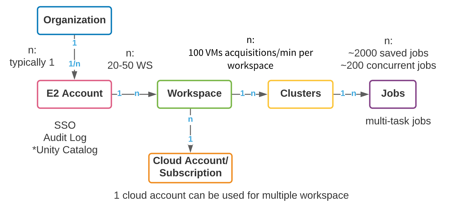
    Introducing the MeshaVerse: Next-Gen Data Mesh 2.0

    $
    0
    0

    At Databricks, we have a (healthy) obsession with building and finding new ways to address our customers’ biggest pain points so that they can unlock new value across all of their data – regardless of their role within an organization. A Data Mesh helps solve some of these challenges by giving teams complete control of their lifecycle while enabling more self-service. The data lakehouse architecture helps organizations drive their Data Mesh journey by enabling a decentralized approach to storing and processing data – while still centralizing security, governance, and discovery.

    That’s why today, we’re thrilled to introduce MeshaVerse, a Lakehouse-powered data mesh that gives you full, interactive control over your data via a VR-driven experience. MeshaVerse introduces a new augmented reality layer on top of your data in Delta Lake via rentable rooms in your Virtual Lakehouse. To get started, all you need is a virtual clone of your Delta Lake data using:

    CREATE ROOM sales_data
    VIRTUAL CLONE source_table_name
    LOCATION MeshaVerse/room

    MeshaVerse completely abstracts your data from your cloud-based Lakehouse. No data or metadata is actually stored within the MeshaVerse – no more data security challenges or compliance nightmares.

    Virtual domain data as a product

    On a path to the Data Mesh, we find that many data teams still struggle with discovering and consuming siloed data. To address this, we are shifting to virtual data in a virtual distributed domain-driven architecture.

    With the development of a MeshaVerse connector, our engineers built virtual abstracted data rooms of the Lakehouse via an augmented data reality experience across the architectural quantum. This enables data teams to build full abstractions of their data into a virtual data set, creating virtual domain data that can then be consumed using vendor-agnostic VR headsets or smartglasses.

    Virtual domain data as a product helps data teams apply rigor to data sets by meeting the following requirements:

    • Discoverable: In a virtual room, data can be discovered using the MeshaVerse VR smartglasses. Via an interactive experience, data scientists, data engineers, and developers can explore virtual data sets with their hands.
    • Addressable: Users can rent rooms in the Lakehouse, making the data directly addressable by their room number.
    • Shareable: Collaboration is core to Databricks. With MeshaVerse, data practitioners can meet in the rooms to explore and share polyglot delta products.
    • Secure: With no data accessible or usable within the MeshaVerse – even with role-based room key cards – security is impenetrable. Minimize security threats while also streamlining regulatory compliance.

    How it works

    When designing MeshaVerse, our primary focus was on preserving decentralization while ensuring data reliability, data quality, and scale. Our novel approach includes implementing Dymlink, a symlink in the data lakehouse, and a new SlinkSync (Symbolic link Sync), a symlink that links Dymlinks together – similar to a linked list.

    By establishing which symlinks can be composed as a set – using either a direct probable or indirect inverse probable match – we are able to infer the convergence criteria of a nondivergent series (i.e the compressed representation of the data) while always ensuring we stay within the gradient of the curve. As a result, we’re able to prevent an infinite recursion that can potentially stale all data retrieval from the Data Mesh. Stay tuned for a future blog, where we’ll dive deeper into this approach.

    The integrity of this virtual data is ensured in real-time and at scale using a more recent implementation of Databricks Brickchain, taking advantage of all global compute power and therefore offering the potential to store the entire planet’s data with a fraction of the footprint.

    MeshaVerse principles

    Data Mesh’s utility is largely due to its core operating principles. In alignment with this approach, we’ve developed our own set of MeshaVerse principles designed to empower data teams and simplify virtual data use cases:

    Augmented data ownership and architecture
    Domain data that reside in the MeshaVerse is enhanced by MeshaVerse AR-generated perceptual information, sometimes across multiple sensory modalities, including visual, auditory, haptic, somatosensory and olfactory. MeshaVerse AR can be defined as a system that incorporates three basic features: a combination of real data and virtual data, real-time analytics, and accurate 3D registration of virtual data.

    Data as a shortcut
    Data explosion is real. As businesses accrue exponentially more data, they are faced with data swamps and scaling challenges. The MeshaVerse is systematically designed to reduce the need for data streaming and pipeline building. Via our VR goggles, see eye to eye with your data. Even when all of it is not readily available. No coding required.

    Self-serve experience
    With an Airbnb-like experience, rent a room inside the MeshaVerse. Either solo or with your entire data team for even more streamlined collaboration. Choose from a selection of pre-designed Lakehouse settings.

    Federated computational governance
    Symlink representations of your data are stored as cryptographic hashes in a brick within the Brickchain, making it possible for any participating party to validate that the data is completely secure. In a peer-to-peer network of distributed ledgers in the Brickchainmetadata is governed in a federated architecture.

    What’s next

    The MeshaVerse is the next evolution of the Databricks Lakehouse and accelerates our vision to make Databricks simple, open and multi-reality. That’s why we’ll be launching a new research and development office dedicated to the MeshaVerse. Stay tuned for more details!

    --

    Try Databricks for free. Get started today.

    The post Introducing the MeshaVerse: Next-Gen Data Mesh 2.0 appeared first on Databricks.
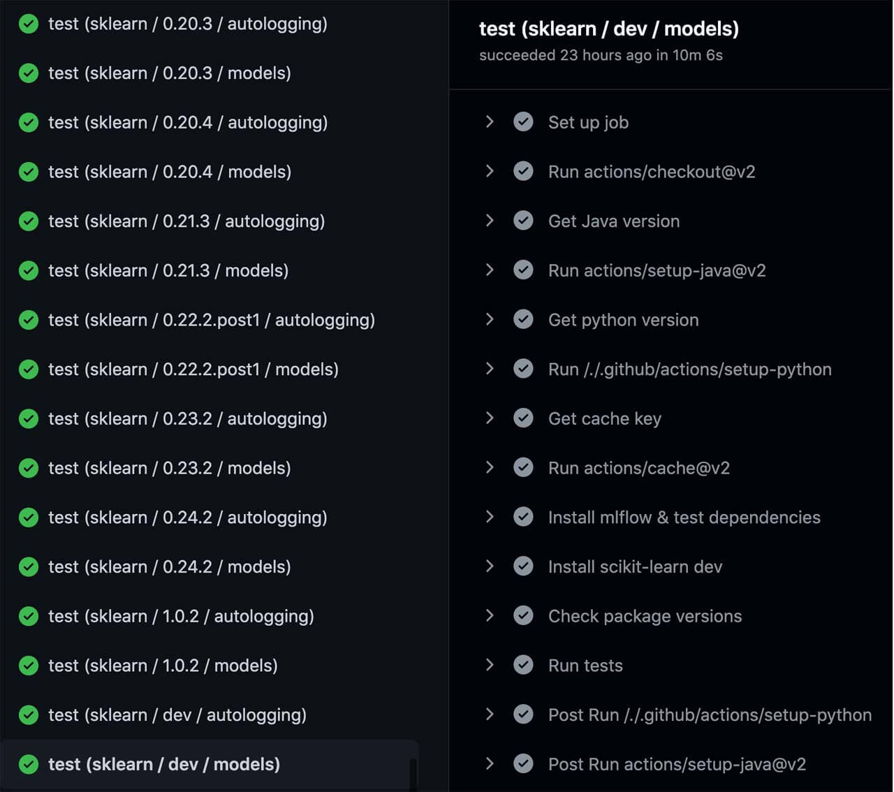
    Announcing Generally Availability of Databricks’ Delta Live Tables (DLT)

    $
    0
    0

    Today, we are thrilled to announce that Delta Live Tables (DLT) is generally available (GA) on the Amazon AWS and Microsoft Azure clouds, and publicly available on Google Cloud! In this blog post, we explore how DLT is helping data engineers and analysts in leading companies easily build production-ready streaming or batch pipelines, automatically manage infrastructure at scale, and deliver a new generation of data, analytics, and AI applications.

    Customers win with simple streaming and batch ETL on the Lakehouse

    Processing streaming and batch workloads for ETL is a fundamental initiative for analytics, data science and ML workloads – a trend that is continuing to accelerate given the vast amount of data that organizations are generating. But processing this raw, unstructured data into clean, documented, and trusted information is a critical step before it can be used to drive business insights. We’ve learned from our customers that turning SQL queries into production ETL pipelines typically involves a lot of tedious, complicated operational work. Even at a small scale, the majority of a data engineer’s time is spent on tooling and managing infrastructure rather than transformation. We also learned from our customers that observability and governance were extremely difficult to implement and, as a result, often left out of the solution entirely. This led to spending lots of time on undifferentiated tasks and led to data that was untrustworthy, not reliable, and costly.

    This is why we built Delta LiveTables, the first ETL framework that uses a simple declarative approach to building reliable data pipelines and automatically managing your infrastructure at scale so data analysts and engineers can spend less time on tooling and focus on getting value from data. DLT allows data engineers and analysts to drastically reduce implementation time by accelerating development and automating complex operational tasks.

    Delta Live Tables is already powering production use cases at leading companies around the globe. From startups to enterprises, over 400 companies including ADP, Shell, Jumbo, Bread Finance, JLL and more have used DLT to power the next generation of self-served analytics and data applications:

    • ADP: “At ADP, we are migrating our human resource management data to an integrated data store on the Lakehouse. Delta Live Tables has helped our team build in quality controls, and because of the declarative APIs, support for batch and real-time using only SQL, it has enabled our team to save time and effort in managing our data.” – Jack Berkowitz, Chief Data Officer – ADP
    • Audantic: “Our goal is to continue to leverage machine learning to develop innovative products that expand our reach into new markets and geographies. Databricks is a foundational part of this strategy that will help us get there faster and more efficiently. Delta Live Tables is enabling us to do some things on the scale and performance side that we haven’t been able to do before. We now run our pipelines on a daily basis compared to a weekly or even monthly basis before — that’s an order of magnitude improvement.” – Joel Lowery, Chief Information Officer – Audantic
    • Shell: “At Shell, we are aggregating all our sensor data into an integrated data store. Delta Live Tables has helped our teams save time and effort in managing data at [the multi-trillion-record scale] and continuously improving our AI engineering capability. With this capability augmenting the existing lakehouse architecture, Databricks is disrupting the ETL and data warehouse markets, which is important for companies like ours. We are excited to continue to work with Databricks as an innovation partner.” – Dan Jeavons, General Manager Data Science – Shell
    • Bread Finance: “Delta Live Tables enables collaboration and removes data engineering resource blockers, allowing our analytics and BI teams to self-serve without needing to know Spark or Scala. In fact, one of our data analysts — with no prior Databricks or Spark experience — was able to build a DLT pipeline to turn file streams on S3 into usable exploratory datasets within a matter of hours using mostly SQL.” – Christina Taylor, Senior Data Engineer – Bread Finance

    Modern software engineering for ETL processing

    DLT allows analysts and data engineers to easily build production-ready streaming or batch ETL pipelines in SQL and Python. It simplifies ETL development by uniquely capturing a declarative description of the full data pipelines to understand dependencies live and automate away virtually all of the inherent operational complexity. With DLT, engineers can concentrate on delivering data rather than operating and maintaining pipelines, and take advantage of key benefits:

    • Accelerate ETL development: Unlike solutions that require you to manually hand-stitch fragments of code to build end-to-end pipelines, DLT makes it possible to declaratively express entire data flows in SQL and Python. In addition, DLT natively enables modern software engineering best practices like the ability to develop in environment(s) separate from production, the ability to easily test it before deploying, deploy and manage environments using parameterization, unit testing and documentation. As a result, you can simplify the development, testing, deployment, operations and monitoring of ETL pipelines with first-class constructs for expressing transformations, CI/CD, SLAs and quality expectations, and seamlessly handling batch and streaming in a single API.
    • Automatically manage infrastructure: DLT was built from the ground-up to automatically manage your infrastructure and automate complex and time-consuming activities. Sizing clusters for optimal performance given changing, unpredictable data volumes can be challenging and lead to overprovisioning. DLT automatically scales compute to meet performance SLAs by providing the user with the option to set the minimum and maximum number of instances and let DLT size up the cluster according to cluster utilization. In addition, tasks like orchestration, error handling and recovery, and performance optimization are all handled automatically. With DLT, you can focus on data transformation instead of operations.
    • Data confidence: Deliver reliable data with built-in quality controls, testing, monitoring and enforcement to ensure accurate and useful BI, Data Science, and ML. DLT makes it easy to create trusted data sources by including first-class support for data quality management and monitoring tools using a feature called Expectations. Expectations help prevent bad data from flowing into tables, track data quality over time, and provide tools to troubleshoot bad data with granular pipeline observability so you get a high-fidelity lineage diagram of your pipeline, track dependencies, and aggregate data quality metrics across all of your pipelines.
    • Simplified batch and streaming: Provide the freshest/up-to-date data for apps with data self-optimized and auto-scaling data pipelines for batch or streaming processing and choose optimal cost-performance. Unlike other products that force you to deal with streaming and batch workloads separately, DLT supports any type of data workload with a single API so data engineers and analysts alike can build cloud-scale data pipelines faster and without needing to have advanced data engineering skills.

     Databricks’ Delta Live Tables dashboard, now available on AWS, Azure Databricks, and Google Cloud.

    Since the preview launch of DLT, we have enabled several enterprise capabilities and UX improvements. We have extended our UI to make it easier to schedule DLT pipelines, view errors, manage ACLs, improved table lineage visuals, and added a data quality observability UI and metrics. In addition, we have released support for Change Data Capture (CDC) to efficiently and easily capture continually arriving data, as well as launched a preview of Enhanced Auto Scaling that provides superior performance for streaming workloads.

    Get started with Delta Live Tables on the Lakehouse

    Watch the demo below to discover the ease of use of DLT for data engineers and analysts alike:

    If you already are a Databricks customer, simply follow the guide to get started. Read the release notes to learn more about what’s included in this GA release. If you are not an existing Databricks customer, sign up for a free trial and you can view our detailed DLT Pricing here.

    What’s next

    Sign up for our Delta Live Tables Webinar with Michael Armbrust and JLL on April 14th to dive in and learn more about Delta Live Tables at Databricks.com.

    --

    Try Databricks for free. Get started today.

    The post Announcing Generally Availability of Databricks’ Delta Live Tables (DLT) appeared first on Databricks.
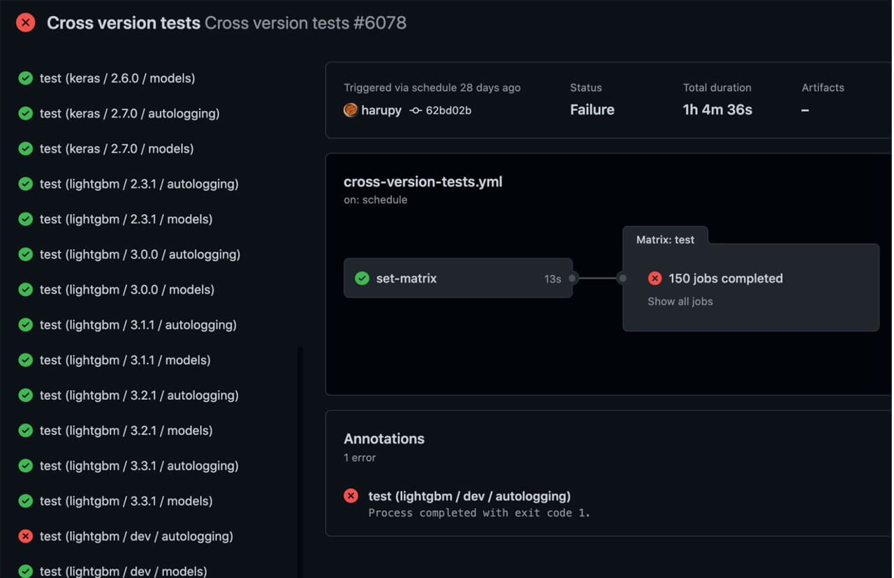
    Viewing all 1874 articles
    Browse latest View live