Quantcast
Channel: Databricks
Viewing all 1999 articles
Browse latest View live

100x Faster Bridge between Apache Spark and R with User-Defined Functions on Databricks

$
0
0

SparkR User-Defined Function (UDF) API opens up opportunities for big data workloads running on Apache Spark to embrace R’s rich package ecosystem. Some of our customers that have R experts on board use SparkR UDF API to blend R’s sophisticated packages into their ETL pipeline, applying transformations that go beyond Spark’s built-in functions on the distributed SparkDataFrame. Some other customers use R UDFs for parallel simulations or hyper-parameter tuning. Overall, the API is powerful and enables many use cases.

SparkR UDF API transfers data between Spark JVM and R process back and forth. Inside the UDF function, user gets a wonderful island of R with access to the entire R ecosystem. But unfortunately, the bridge between R and JVM is far from efficient. It currently only allows one “car” to pass on the bridge at any time, and the “car” here is a single field in any Row of a SparkDataFrame. It should not be a surprise that traffic on the bridge is very slow.

In this blog, we provide an overview of SparkR’s UDF API and then show how we made the bridge between R and Spark on Databricks efficient. We present some benchmark results.

Overview of SparkR User-Defined Function API

SparkR offers four APIs that run a user-defined function in R to a SparkDataFrame

  • dapply()
  • dapplyCollect()
  • gapply()
  • gapplyCollect()

dapply() allows you to run an R function on each partition of the SparkDataFrame and returns the result as a new SparkDataFrame, on which you may apply other transformations or actions. gapply() allows you to apply a function to each grouped partition consisting of a key and the corresponding rows in a SparkDataFrame. dapplyCollect() and gapplyCollect() are shortcuts if you want to call collect() on the result.

The following diagram illustrates the serialization and deserialization performed during the execution of the UDF. The data gets serialized twice and deserialized twice in total, all of which are row-wise.

By vectorizing data serialization and deserialization in Databricks Runtime 4.3, we encode and decode all the values of a column at once. This eliminates the primary bottleneck which row-wise serialization, and significantly improves SparkR’s UDF performance. Also, the benefit from the vectorization is more drastic for larger datasets.

Methodology and Benchmark Results

We use the Airlines’ dataset for the benchmark. The dataset consists of 24 integer fields and 5 string fields including date, departure time, destination and other information about each flight. We measure the running time and throughput of SparkR UDF APIs on subsets of data with varying sizes on both Databricks Runtime (DBR) 4.2 and Databricks Runtime 4.3, and report the mean and standard deviation over 20 runs. DBR 4.3 includes the new optimization work, while DBR 4.2 does not. All the tests are performed on cluster with eight i3.xlarge workers.

SparkR::dapply()

To demonstrate the acceleration, we use a trivial user function with SparkR::dapply() that simply returns the input R data.frame.

Overall, the improvement is one to two orders of magnitude, and increases with the number of rows in the dataset. For data with 800k rows, the running time reduces from more than 100s to less than 3s. The throughput of DBR 4.3 is more than 30 MB/s, while it is only about 0.5 MiB/s before our optimization. For data with 6M rows, the running time is still below 10 seconds, and the throughput is about 70 MiB/s — that is 100x acceleration!

SparkR::gapply()

In practice SparkR::gapply() is more frequently used compared to dapply(). In our benchmarks, we removed the shuffling cost by pre-partitioning the data by the DayOfMonth field, and using the same key in gapply() to count the total number of flights on each day of month.

In our experiment, gapply() runs faster than dapply(), because the output data of the UDF is the aggregated result of the input data, which is small. Thus the total serialization and deserialization time could be halved.

Summary

In summary, our optimization has an overwhelming advantage over the previous version on all ranges of typical data sizes, and for larger data, we observed one to two orders of magnitude improvement. Such significant improvement can empower many use cases that were barely acceptable before. Also, Date and Timestamp data types are now supported in DBR 4.3, which had to be cast to double in the previous version.

Read More

This optimization is one of a series of efforts from Databricks that boost the performance of SparkR on Databricks Runtime. Check out the following assets for more information:

--

Try Databricks for free. Get started today.

The post 100x Faster Bridge between Apache Spark and R with User-Defined Functions on Databricks appeared first on Databricks.


Introducing mlflow-apps: A Repository of Sample Applications for MLflow

$
0
0

Introduction

This summer, I was a software engineering intern at Databricks on the Machine Learning (ML) Platform team. As part of my intern project, I built a set of MLflow apps that demonstrate MLflow’s capabilities and offer the community examples to learn from.

In this blog, I’ll discuss this library of pluggable ML applications, all runnable via MLflow. In addition, I’ll share how I implemented two MLflow features during my internship: running MLprojects from Git subdirectories and TensorFlow integration.

mlflow-apps: A Set of Sample MLflow Applications

mlflow-apps is a repository of pluggable ML applications runnable via MLflow. It helps users get a jump start on using MLflow by providing concrete examples on how MLflow can be used.

Through a one-line MLflow API call or CLI commands, users can run apps to train TensorFlow, XGBoost, and scikit-learn models on data stored locally or in cloud storage. These apps log common metrics and parameters via MLflow’s tracking APIs, allowing users to easily compare fitted models.

Currently, mlflow-apps focuses on model training, but we plan to add additional functionality for feature engineering /data pre-processing. We welcome community contributions on this front.

mlflow-apps comprises of three apps, each of which creates and trains a different model based on your input data. The models trained by the apps are:

Curious about how you can use the apps? You can see the source code and a short tutorial for the apps in the repository here. For an in-depth tutorial that demonstrates how to use these apps with MLflow within Databricks, check out this notebook.

Enhancing Open Source MLflow

MLflow has the ability to run MLflow projects located in remote git repositories, via CLI commands such as

mlflow run git@github.com:example/example.git ...

MLflow can now execute ML projects described by MLproject files located in subdirectories of git repositories. Previously, executing an MLflow run from a remote repository required the MLproject and conda.yaml files to be in the root directory of the git repository. An example git repo structure would have had to look like the following:

Original MLFlow Git Repo Layout

This git repo structure would cause each project to share unnecessary dependencies with each other (e.g. running the sklearn_file would require a conda environment with all three different frameworks installed despite only sklearn being needed). With the new feature implemented, a command could look like this:

mlflow run git@github.com:example/example.git#sklearn_project ...

which would subsequently access the MLproject file located in a subdirectory called sklearn_project. The previous example git repo shown above can now be restructured as such:

Improved MLflow Project Git Layout

Now, the projects and dependencies are nicely modularized and decoupled (e.g. sklearn_project only needs the sklearn framework when creating a conda environment). This in turn leads to a cleaner and easier user experience with MLflow.

TensorFlow Integration for MLflow

Although MLflow allows users to run and deploy models using any ML library, we also want the project to have built-in easy-to-use integrations with popular libraries. As part of my internship, I developed an integration for TensorFlow, which allows saving, loading and deploying TensorFlow models.

# Saving TensorFlow model.
saved_estimator_path = estimator.export_savedmodel(saved_estimator_path,
                            receiver_fn).decode("utf-8")
# Logging the TensorFlow model just saved.
mlflow.tensorflow.log_saved_model(saved_model_dir=saved_estimator_path,
                             signature_def_key="predict",
                             artifact_path=tmp.path("model"))

In addition to logging TensorFlow models, you can load them back and perform inference on them using MLflow APIs.

# Loading the model back as a Python Function
pyfunc = mlflow.tensorflow.load_pyfunc(mlflow.tracking._get_model_log_dir(model_name=path, 
                                      run_id=run_id))
# predict with new or test data
predictions = pyfunc.predict(test_df)

MLflow currently has built-in integrations for TensorFlow, SparkML, H2O, and sklearn models. Keep your eye out for more framework support in the near future!

Conclusion

While working on mlflow-apps, I was able to experience MLflow both as a user and a project developer. I was able to better see the how closely intertwined the community and project developers are for open source projects like MLflow.

As my first internship, I couldn’t have asked for a better experience. I came into Databricks eager to learn everything about the industry and new technologies – what I found were engineers who matched my desire to learn. Because I was in an environment where accomplished engineers constantly push themselves to learn and challenge themselves, I, in turn, was encouraged to do the same. Consequently, I improved my skills both as a software engineer by leaps and bounds.

Special shoutout to the Production Serving and ML Platform teams, which include Matei Zaharia, Aaron Davidson, Paul Ogilvie, Andrew Chen, Mani Parkhe, Tomas Nykodym, Sue Ann Hong, Corey Zumar, and my mentor Sid Murching. Thanks for the fantastic summer!

Read More

Check out other resources for learning about MLflow & mlflow-apps here:

--

Try Databricks for free. Get started today.

The post Introducing mlflow-apps: A Repository of Sample Applications for MLflow appeared first on Databricks.

New Features in MLflow v0.5.1 Release

$
0
0

Today, we’re excited to announce MLflow v0.5.0 and MLflow v0.5.1, which were released last week with some new features. MLflow 0.5.1 is already available on PyPI and docs are updated. If you do pip install mlflow as described in the MLflow quickstart guide, you will get the recent release.

In this post, we’ll describe new features and fixes in this release.

Keras and PyTorch Model Integration

As part of MLflow 0.5.1 and continued effort to offer a range of machine learning frameworks, we’ve extended support to save and load Keras and PyTorch models using log_model APIs. These model flavors APIs export their models in their respective formats, so either Keras or PyTorch applications can reuse them, not only from MLflow but natively from Keras or PyTorch code too.

Using Keras Model APIs

Once you have defined, trained, and evaluated your Keras model, you can log the model as part of an MLflow artifact as well as export the model in Keras HDF5 format for others to load it or serve it for predictions. For example, this Keras snippet code shows how:

from keras import Dense, layers
import mlflow 

# Build, compile, and train your model
keras_model = ...
keras_model.compile(optimizer=’rmsprop’, loss=’mse’, metrics[‘accuracy’])
results = keras_model.fit(x_train, y_train, epochs=20, batch_size = 128, validation_data=(x_val, y_val))
...
# Log metrics and log the model
with mlflow.start_run() as run:
   ...
   mlflow.keras.log_model(keras_model, “keras-model”)

# Load the model as Keras model or as pyfunc and use its predict() method

keras_model = mlflow.keras.load_model(“keras-model”, run_id=”96771d893a5e46159d9f3b49bf9013e2”)
predictions = keras_model.predict(x_test)
...

Using PyTorch Model APIs

Similarly, you can use the model APIs to log models in PyTorch, too. For example, the code snippets below are similar in PyTorch, with minor changes in how PyTorch exposes its methods. However, with pyfunc the method is the same: predict():

import mlflow 
import pytorch

# Build, compile, and train your model
pytorch_model = ...
pytorch_model.train()
pytorch_model.eval()
...
y_pred = pytorch_model.model(x_data)

# Log metrics and log the model
with mlflow.start_run() as run:
...
   mlflow.pytorch.log_model(pytorch_model, “pytorch-model”)
   # Load the model as pytorch model or as pyfunc and use its predict() method

pytorch_model = mlflow.pytorch.load_model(“pytorch-model”)
y_predictions = pytorch_model.model(x_test)

Python APIs for Experiment and Run Management

To query past runs and experiments, we added new public APIs as part of mlflow.tracking module. In the process, we have also refactored the old APIs into mlflow module for logging parameters and metrics for current runs. So for example, to log basic parameters and metrics for the current run, you can use the mlflow.log_xxxx() calls.

import mlflow
uu_id = ‘v.0.5’
with mflow.start_run(run_uuid=uu_id) as run:
   mflow.log_param(“game”, 1)
   mlflow.log_metric(“score”, 25)
   ...

However, to access this run’s results, say in another part of application, you can use mflow.tracking APIs as such:

import mlflow.tracking

#get the service; defaults to URI or locally from ‘mlruns’
run_uuid = ‘v.0.5’
run = mlflow.tracking.get_service().get_run(run_uuid)
score = run.data.metrics[0]

While the former deals with persisting metrics, parameters and artifacts for the currently active run, the latter allows managing experiments and runs (especially historical runs).

With this new APIs, developers have access to Python CRUD interface to MLflow Experiments and Runs. Because it is a lower level API, it maps well to REST calls. As such you can build a REST-based service around your experimental runs.

UI Improvements for Comparing Runs

Thanks to Toon Baeyens (Issue #268, @ToonKBC), in the MFlow Tracking UI we can compare two runs with a scatter plot. For example, this image shows a number of trees and its corresponding rmse metric.

Also, with better columnar and tabular presentation and organization of experimental runs, metrics, and parameters, you can easily visualize the outcomes and compare runs. Together with navigation breadcrumbs, the overall encounter is a better UI experience.

Other Features and Bug Fixes

In addition to these features, other items, bugs and documentation fixes are included in this release. Some items worthy of note are:

  • [Sagemaker] Users can specify a custom VPC when deploying SageMaker models (#304, @dbczumar)
  • [Artifacts] SFTP artifactory store added (#260, @ToonKBC)
  • [Pyfunc] Pyfunc serialization now includes the Python version and warns if the major version differs (can be suppressed by using load_pyfunc(suppress_warnings=True)) (#230, @dbczumar)
  • [Pyfunc] Pyfunc serve/predict will activate conda environment stored in MLModel. This can be disabled by adding --no-conda to mlflow pyfunc serve or mlflow pyfunc predict (#225, @0wu)
  • [CLI] mlflow run can now be run against projects with no conda.yaml specified. By default, an empty conda environment will be created — previously, it would just fail. You can still pass --no-conda to avoid entering a conda environment altogether (#218, @smurching)
  • Fix with mlflow.start_run() as run to actually set run to the created Run (previously, it was None) (#322, @tomasatdatabricks)
  • [BUG-FIXES] Fixes to DBFS artifactory to throw an exception if logging an artifact fails (#309) and to mimic FileStore’s behavior of logging subdirectories (#347, @andrewmchen)
  • [BUG-FIXES] Fix spark.load_model not to delete the DFS tempdir (#335, @aarondav)
  • [BUG-FIXES] Make Python API forward-compatible with newer server versions of protos (#348, @aarondav)
  • [UI] Improved API docs (#305, #284, @smurching)

The full list of changes and contributions from the community can be found in the 0.5.1 Changelog. We welcome more input on mlflow-users@googlegroups.com or by filing issues or submitting patches on GitHub. For real-time questions about MLflow, we’ve also recently created a Slack channel for MLflow as well as you can follow @MLflowOrg on Twitter.

Credits

MLflow 0.5.1 includes patches, bug fixes, and doc changes from Aaron Davidson, Adrian Zhuang, Alex Adamson, Andrew Chen, Arinto Murdopo, Corey Zumar, Jules Damji, Matei Zaharia, @RBang1, Siddharth Murching, Stephanie Bodoff, Tomas Nykodym, Tingfan Wu, Toon Baeyens, and Yassine Alouini.

--

Try Databricks for free. Get started today.

The post New Features in MLflow v0.5.1 Release appeared first on Databricks.

How to Use MLflow to Experiment a Keras Network Model: Binary Classification for Movie Reviews

$
0
0

In the last blog post, we demonstrated the ease with which you can get started with MLflow, an open-source platform to manage machine learning lifecycle. In particular, we illustrated a simple Keras/TensorFlow model using MLflow and PyCharm. This time we explore a binary classification Keras network model. Using MLflow’s Tracking APIs, we will track metrics—accuracy and loss–during training and validation from runs between baseline and experimental models. As before we will use PyCharm and localhost to run all experiments.

Binary Classification for IMDB Movie Reviews

Binary classification is a common machine learning problem, where you want to categorize the outcome into two distinct classes, especially for sentiment classification. For this example, we will classify movie reviews into “positive” or “negative” reviews, by examining review’s text content for occurance of common words that express an emotion.

Borrowed primarily from François Chollet’s “Deep Learning with Python”, the Keras network example code has been modularized and modified to constitute as an MLFlow project and incorporate the MLflow Tracking API to log parameters, metrics, and artifacts.

Methodology and Experiments

The Internet Movie Database (IMDB) comes packaged with Keras; it is a set of 50,000 popular movies, split into 25,000 reviews for training and 25,000 for validation, with an even distribution of “positive” and “negative” sentiments. We will use this dataset for training and validating our a model.

By simple data preparation, we can convert this data into tensors, as numpy arrays, for our Keras neural network model to process. (The code for reading and preparing data is in the module: data_utils_nn.py.)

We will create two Keras neural network models—baseline and experimental—and train them on our dataset. While the baseline model will remain constant, we will experiment with the two experimental models, by supplying different tuning parameters and loss functions to compare the results.

This is where MLflow’s tracking component immensely helps us evaluate which of the myriad tunning parameters produce the best metrics in our models. Let’s first examine the baseline model.

Baseline Model: Keras Neural Network Performance

source : Deep Learning with Python

François’s code example employs this Keras network architectural choice for binary classification. It comprises of three Dense layers: one hidden layer (16 units), one input layer (16 units), and one output layer (1 unit), as show in the diagram. “A hidden unit is a dimension in the representation space of the layer,” Chollet writes, where 16 is adequate for this problem space; for complex problems, like image classification, we can always bump up the units or add hidden layers to experiment and observe its effect on accuracy and loss metrics (which we shall do in the experiments below).

While the input and hidden layers use relu as an activation function, the final output layer uses sigmoid, to squash its results into probabilities between [0, 1]. Anything closer to 1 suggests positive, while something below 0.5 can indicate negative.

With this recommended baseline architecture, we train our base model and log all the parameters, metrics, and artifacts. This snippet code, from module models_nn.py, creates a stack of dense layers as depicted in the diagram above.

....
def build_basic_model(self):
 base_model = models.Sequential()
 base_model.add(layers.Dense(16, activation='relu', input_shape=(10000,)))
 base_model.add(layers.Dense(16, activation='relu'))
 base_model.add(layers.Dense(1, activation='sigmoid'))

 return base_model

Next, after building the model, we compile the model, with appropriate loss function and optimizers. Since we are expecting probabilities as our final output, the recommended loss function for binary classification is binary_crosstropy and the corresponding suggested optimizer is rmsprop. The code snippet from module train_nn.py compiles our model.

from keras import optimizers
 ...
 ... 
if optimizer == 'rmsprop':
   opt = optimizers.RMSprop(lr=lr)
model.compile(optimizer=opt, loss=’binary_crossentropy’, metrics=[‘accuracy’])
...

Finally, we fit (train) and evaluate by running iterations or epochs with a default batch size for 512 samples from the IMDB data set for each iteration, with default parameters:

  • Epochs = 20
  • Loss = binary_misantropy
  • Units = 16
  • Hidden Layers = 1

To run from the command line, cd to the Git repository directory keras/imdbclassifier and run either:

python main_nn.py

Or from the GitHub repo top level directory run:

mlflow run keras/imdbclassifier -e main

Or directly from Gitbub:

mlflow run 'https://github.com/dmatrix/jsd-mlflow-examples.git#keras/imdbclassifier'

Fig 1: Animated run with base model parameters on a local host

At the end of the run, the model will print a set of final metrics such as binary_loss, binary_accuracy, validation_loss, and validation_accuracy for both training set and validation set after all iterations.

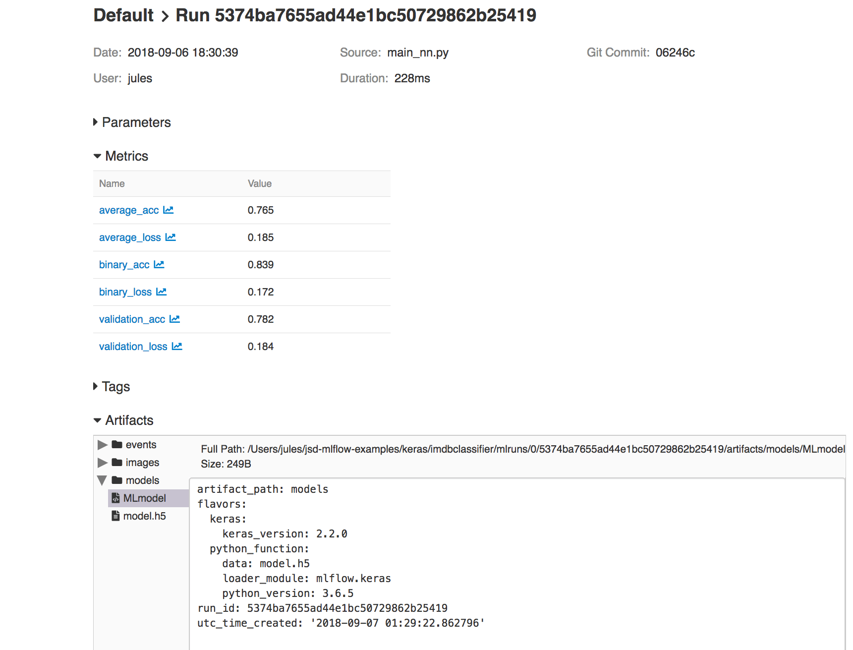
Fig 2: Results and metrics run with base model parameters

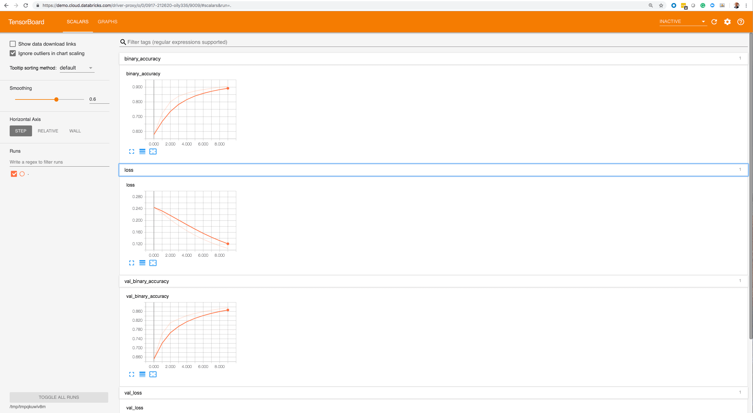
As you will notice from the runs, the loss decreases over iterations while the accuracy increases, with the former converging toward 0 and the latter toward 1.

Our final training data (binary_loss) converged to 0.211 and the validation data (validation_loss) tracked with 0.29—which tracked somewhat closely with binary_loss. On the other hand, the accuracy diverged after several epochs suggesting we may be overfitting with the training data (see plots below).

(Note: To access these plots, launch the MLFlow UI, click on any experimental run, and access its artifacts’ folder.)

When predicting with unseen IMDB reviews, the prediction results averaged at 0.88 accuracy, which is close to our validation accuracy, but still fairly far off. However, as you can see, for some reviews the network confidently predicted results with 99% probability of a positive review.

Fig 3a: Matplotlib artifacts logged with base and experiment model parameters

Fig 3b: Matplotlib artifacts logged with base and experiment model parameters

At this point, after observing the basic model metrics, you may ask, can we do better? Can we tweak some tuning parameters such as number of hidden layers, epochs, loss function or units to affect better results. Let’s try with some recommended experiments.

Experimental Model: Keras Neural Network Performance

MLflow’s Tracking Component allows us to track experimental runs of our model with different parameters and persist their metrics and artifacts for analysis. Let’s launch a couple of runs with the following experimental parameters, as Chollet suggests, that are different from the default model and observe an outcome:

Model Units Epochs Loss Function Hidden Layers
Base 16 20 binary_crosstropy 1
Experiment-1 32 30 binary_crosstropy 3
Experiment-2 32 20 mse 3

Table 1: Models and Parameters

Running Experiments on Local Host

Since we are running MLflow on the local machine, all results are logged locally. However, you can as easily log metrics remotely on a hosted tracking server in Databricks, by simply setting an environment variable MLFLOW_TRACKING_URI or programmatically set with mlflow.set_tracking_uri().

Either connects to a tracking URI and log results. In both cases, the URI can either be a HTTP/HTTPS URI for a remote server, or a local path to a directory. On the local host, the URI defaults to an mlruns directory.

Running Experiments within PyCharm with MLFlow

Since I prefer PyCharm for my Python development, I’ll run my experiments from within PyCharm on my laptop, providing the experimental parameters. Below is an animation from the first experiment. (To learn how to use MLflow within PyCharm read my previous blog).

Although I ran the experiments by providing parameters within PyCharm’s run configurations, you can just as easily run these experiments on the command line from the top level directory, too:

mlflow run keras/imdbclassifier -e main -P hidden_layers=3 -P epochs=30
mlflow run keras/imdbclassifier -e main -P hidden_layers=3 -P output=32 -P loss=mse

Fig 4: Animated run with experiment-1 model parameters

All experiments’ runs are logged, and we can examine each metric and compare various runs to assess results. All the code that logs these artifacts using MLflow Tracking API is in the train_nn.py module. Here is a partial code snippet:

        ....
        with mlflow.start_run():
            # log parameters
            mlflow.log_param("hidden_layers", args.hidden_layers)
            mlflow.log_param("output", args.output)
            mlflow.log_param("epochs", args.epochs)
            mlflow.log_param("loss_function", args.loss)
            # log metrics
            mlflow.log_metric("binary_loss", ktrain_cls.get_binary_loss(history))
            mlflow.log_metric("binary_acc",  ktrain_cls.get_binary_acc(history))
            mlflow.log_metric("validation_loss", ktrain_cls.get_binary_loss(history))
            mlflow.log_metric("validation_acc", ktrain_cls.get_validation_acc(history))
            mlflow.log_metric("average_loss", results[0])
            mlflow.log_metric("average_acc", results[1])

            # log artifacts (matplotlib images for loss/accuracy)
            mlflow.log_artifacts(image_dir)
          #log model
            mlflow.keras.log_model(keras_model, model_dir)

        print("loss function use", args.loss)

if __name__ == '__main__':
    #
    # main used for testing the functions
    #
    parser = KParseArgs()
    args = parser.parse_args()

    flag = len(sys.argv) == 1

    if flag:
        print("Using Default Baseline parameters")
    else:
        print("Using Experimental parameters")

    print("hidden_layers:", args.hidden_layers)
    print("output:", args.output)
    print("epochs:", args.epochs)
    print("loss:", args.loss)
    train_models_cls = KTrain().train_models(args, flag)

Comparing Experiments and Results with MLFlow UI

Now the best part. MLflow allows you to view all your runs and logged results from an MLflow GUI, where you can compare all three runs’ metrics. Recent UI improvements in MLFlow v0.5.1 offer a better experience in comparing runs.

To launch a Flask tracking server on your localhost:5000, use command line mlflow ui.

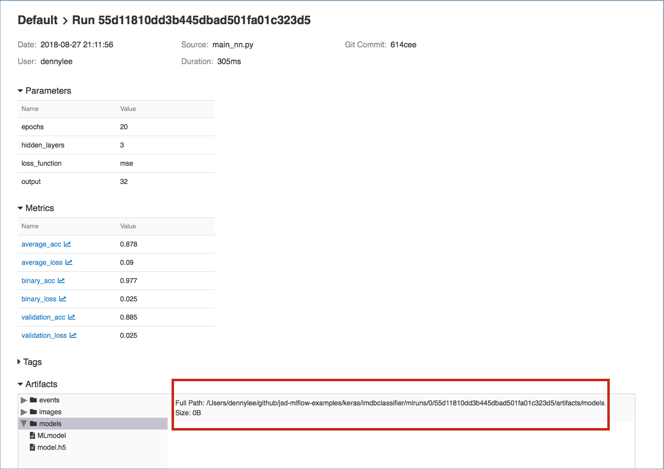
Fig 5: MLflow UI table view of all runs’ metrics, parameters, and artifacts

For example, I can compare all three experiments’ metrics to see which of the runs produced an acceptable validation accuracy and loss as well view each of my experiments’ matplotlib images to see how they fared across epochs.

Fig 6: Animated view of metrics with experimental parameters

Comparing Results from Three Runs

By quickly examining our runs in MLFlow UI, we can easily observe the following:

  • Changing the number of epochs did not give us any benefit except the model began overfitting, as it reached training accuracy of 99%, with no corresponding difference to validation accuracy, which diverges after several epochs.
  • Changing the loss function to mse, units to 32, and hidden layers to 3, however, gave us a better validation loss as well as a converging average_loss to 0 for the validation data. With other metrics tracking closely across models, a couple of extra hidden layers and more units minimized the validation loss.

Fig 7: Comparing three run with parameters

Improving Model Metrics With Further Experiments

Notably, François Chollet posits that with further training, validation, and tests (TVT), we can achieve higher accuracy, over 95% and converge the loss to 0.01%. One way to achieve it is through further experiments with machine learning techniques such as
add more data, simple-hold out validation, k-fold validation, add weight regularization, add dropout network layers, and increase network capacity. These could minimize overfitting and achieve generalization—and as consequence drive better accuracy and minimal loss.

We could implement these techniques here, carry out further experiments, and use MLflow to assess outcomes. I’ll leave that as an exercise for the reader.

Because such experiments and iterations are so central to the way data scientists asses models, MLflow facilitates such lifecycle tasks. To that extent, this blog demonstrated that part of MLflow’s functionality.

Closing Thoughts

So far we demonstrated the key use of MLflow Tracking Component’s APIs to log model’s myriad parameters, metrics, and artifacts so that at any point or anyone can reproduce the results from model’s MLflow Git project repository.

Second, through command line, PyCharm runs, and MLFlow UI, we compared various runs to examine the best metrics, and observed that by altering some parameters, we approached a model that could perhaps be used with acceptable accuracy for doing sentiment classification of IMDB movie reviews based on common words that express positive or negative review. Even better, as noted, we could further improve our models’ outcomes by using suggested machine learning techniques.

Finally, but far importantly, we experimented using MLflow within PyCharm on a local host, but we could just as easily track experiments on a remote server. With MLflow, Numpy, Pandas, Keras, and TensorFlow packages installed as part of our PyCharm Python Virtual Environment, this methodical iteration of model experiments is a vital step in a machine learning model’s life cycle. And the MLflow platform facilitates this crucial step—all from within your favorite Python IDE.

What’s Next

Now that we have compared the baseline model to a couple of experimental models and we have seen MLflow’s merits, what is the next step? Try MLflow at mlflow.org to get started. Or try some of tutorials and examples in the documentation.

Read More

Here are some resources for you to learn more:

--

Try Databricks for free. Get started today.

The post How to Use MLflow to Experiment a Keras Network Model: Binary Classification for Movie Reviews appeared first on Databricks.

Introducing Cluster-scoped Init Scripts

$
0
0

This summer, I worked at Databricks as a software engineering intern on the Clusters team. As part of my internship project, I designed and implemented Cluster-scoped init scripts, improving scalability and ease of use.

In this blog, I will discuss various benefits of Cluster-scoped init scripts, followed by my internship experience at Databricks, and the impact it had on my personal and professional growth.

Cluster-scoped Init Scripts

Init scripts are shell scripts that run during the startup of each cluster node before the Spark driver or worker JVM starts. Databricks customers use init scripts for various purposes such as installing custom libraries, launching background processes, or applying enterprise security policies. These new scripts offer several improvements over previous ones, which are now deprecated.

Init scripts are now part of the cluster configuration

One of the biggest pain points for customers used to be that init scripts for a cluster were not part of the cluster configuration and did not show up in the User Interface. Because of this, applying init scripts to a cluster was unintuitive, and editing or cloning a cluster would not preserve the init script configuration. Cluster-scoped init scripts addressed this issue by including an ‘Init Scripts’ panel in the UI of the cluster configuration page, and adding an ‘init_scripts’ field to the public API. This also allows init scripts to take advantage of cluster access control.

curl -n -X POST -H 'Content-Type: application/json' -d '{
  "cluster_id": "1202-211320-brick1",
  "cluster_log_conf": {
    "dbfs" : {
      "destination": "dbfs:/cluster-logs"
    }
  },
  "init_scripts": [ {
    "dbfs": {
      "destination": "dbfs:/databricks/<directory>/postgresql-install.sh"
    }
  } ]
}' https://<databricks-instance>/api/2.0/clusters/edit

Init scripts now work for jobs clusters

Previous init scripts depended on storing the scripts in a folder with the cluster-name. This prevents them from being used in jobs clusters, where cluster names are generated on the fly. Since Cluster-scoped init scripts are part of the cluster configuration, they can be applied to jobs clusters as wel, with an identical interface via both the UI and API.

Environment variables for init scripts

Init scripts now provide access to certain environment variables that are listed here. This reduces the complexity of many init scripts that require access to information such as whether the node is a driver or executor and the cluster id.

Access Control for init scripts

Users can now provide a DBFS or S3 path for their init scripts, which can be stored at arbitrary locations. When using S3, IAM roles can be used to provide access control for init scripts, protecting against malicious or mistaken access/alteration to the init scripts. Read more details on how to set this up here.

Simplified logging

Logs for Cluster-scoped init scripts are now more consistent with Cluster Log Delivery and can be found in the same root folder as driver and executor logs for the cluster.

Additional cluster events

Init Scripts now expose two new cluster events: INIT_SCRIPTS_STARTED and INIT_SCRIPTS_FINISHED. These help users determine the duration of init scripts execution and provide additional clarity as to the state of the cluster at a given moment.

Conclusion

Working on this project exposed me to the process of designing, implementing and testing a customer-facing feature. I learned how to write robust, maintainable code and evaluate execution semantics. I remember my distributed systems professor claiming that a good design can simplify engineering effort by orders of magnitude, resulting in shorter, cleaner code that is less prone to bugs. However, I never imagined that this point would be driven home just a few months later in an industry setting.

I found Databricks engineers to be extremely helpful, with a constant desire to learn and improve, as well as the patience to teach. The leadership is extremely open with the employees and is constantly looking for feedback, even from the interns. The internship program also had a host of fun activities, as well as educational events that allowed us to learn about other areas of the company (e.g., sales, field engineering, customer success).

Finally, I’d like to thank the clusters team for their encouragement and support throughout my project. A special shout out to my manager Ihor Leshko for always being there when needed, Mike Lin for completely changing the way I approach front-end engineering, and my mentor Haogang Chen for teaching me valuable technical skills that enabled me to graduate from writing simple, working code to building robust, production-ready systems.

--

Try Databricks for free. Get started today.

The post Introducing Cluster-scoped Init Scripts appeared first on Databricks.

A Guide to Apache Spark Use Cases, Streaming, and Research Talks at Spark + AI Summit Europe

$
0
0

For much of Apache Spark’s history, its capacity to process data at scale and capability to unify disparate workloads has led Spark developers to tackle new use cases. Through innovation and extension of its ecosystem, developers combine data and AI to develop new applications.

So it befits developers to come to this summit not just to hear about innovations from contributors—but to share their use cases, experiences, research, absorb knowledge, and explore new frontiers.

In this final blog, we shift our focus to these developers who make a difference, not only in their contributions to the Apache Spark ecosystem but also in use of Spark at scale in respective industries.

Let’s start with CERN’s Next Generation Data Analysis Platform with Apache Spark. Enric Tejedor from CERN will share how Spark is used at scale to process exabyte of data from the Large Hadron Collider (LHC) in innovative ways. Similarly, Daniel Lanza of CERN will also discuss Stateful Structure Streaming and Markov Chains Join Forces to Monitor the Biggest Storage of Physics Data. Two fascinating talks that will demonstrate the Spark’s scope and scalability.

“Traditional data architectures are not enough to handle the huge amounts of data generated from millions of users,” writes Ricardo Fanjul of Letgo. Learn from his talk on why and how Spark is used in Designing a Horizontally Scalable Event-Driven Big Data Architecture with Apache Spark.

From atomic particles’ collision data in physical sciences to genomic data in life sciences, Spark is there to process data at scale. Thanks to advancement in unified analytics at scale, in particular, Spark’s ability to process distributed data and because of cheap cloud storage, Spark enters new frontiers in Health and Life Sciences. Databricks’ Henry Davidge will share: Scaling Genomics on Apache Spark by 100x.

Hearing from engineers who undertake migrating workloads from one architecture to another, in favor of Spark, is always insightful. Three speakers will chart their Spark migratory journeys: first, learn from Manuele Bardelli (OLX) as he will chart his technical migratory journey in his talk, “All-at-Once, Once-a-Day” to “A-Little-Each-Time, All-the-Time”; second, Matteo Pelati (DBS bank) will share his Spark journey: Migrating from RDBMS Data Warehouses to Apache Spark; and finally, Yucai Yu (eBay) will discuss Experience of Optimizing Spark SQL When Migrating from Teradata.

Research heralds technology shifts and innovation: at CERN it led to WWW; at Google, it led to TensorFlow and more; at UC Berkeley AMPLab, it led to Apache Spark. Two research sessions may interest you: Accelerating Apache Spark with FPGAs: A Case Study for 10TB TPCx-HS Spark Benchmark Acceleration with FPGA (Intel) and Spark-MPI: Approaching the Fifth Paradigm (NSLS-II). Continuously processing time-series data using Spark is one of many use cases. To address how to use it with Spark, Liang Zhang (Worcester Polytechnic Institute) will share his research work, Spark-ITS: Indexing for Large-Scale Time Series Data on Spark.

We take flying for granted just as we do driving. But what of the machinery that propels us to our desired destinations? Over time they tire. How do you monitor or detect or predict preventive maintenance? Messrs Peter Knight and Honor Powrie (both from GE) will show how to monitor engines in their talk, GE Aviation Spark Application – Experience Porting Analytics into PySpark ML Pipelines.

Uber’s ride-sharing service is as ubiquitous in a global city as its skyscraper skyline. Learn how Uber uses Apache Spark for running hundreds of thousands of analytical queries every day with their Hudi Platform, built with Spark. Messrs Nishith Agarwal and Vinoth Chandar (both from Uber) will discuss this use case in their talk: Hudi: Near Real-Time Spark Pipelines at Petabyte Scale

Finally, two structured streaming and machine learning related use cases of notable interest: First, from Vedant Jain (Databricks), A Microservices Framework for Real-Time Model Scoring Using Structured Streaming; and second, from Heitor Murilo Gomes (LIAAD) and Albert Bifet (LTCI, Telecom ParisTech), Streaming Random Forest Learning in Spark and StreamDM.

What’s Next?

Take advantage of this promo code JulesPicks for a 20% discount and register now!
Come and find out what’s new with Apache Spark, Data, and AI. We hope to see you in London

Read More

--

Try Databricks for free. Get started today.

The post A Guide to Apache Spark Use Cases, Streaming, and Research Talks at Spark + AI Summit Europe appeared first on Databricks.

Building the Fastest DNASeq Pipeline at Scale

$
0
0

Unified Analytics Platform for Genomics

In June, we announced the Unified Analytics Platform for Genomics with a simple goal: accelerate discovery with a collaborative platform for interactive genomic data processing, analytics and AI at massive scale.  In this post, we’ll go into more detail about one component of the platform: a scalable DNASeq pipeline that is concordant with GATK4 at best-in-class speeds.

Making Sense of Sequence Data at Scale

The vast majority of genomic data comes from massively parallel sequencing technology. In this technique, the sample DNA must first be sliced into short segments with lengths of about 100 base pairs. The sequencer will emit the genetic sequence for each segment. In order to correct for sequencing errors, we typically require that each position in the genome is covered by at least 30 of these segments. Since there are about 3 billion base pairs in the human genome, that means that after sequencing, we must reassemble 3 billion / 100 * 30 = 900 million short reads before we can begin real analyses. This is no small effort.

Since this process is common to anyone working with DNA data, it’s important to codify a sound approach. The GATK team at the Broad Institute has led the way in describing best practices for processing DNASeq data, and many people today run either the GATK itself or GATK-compliant pipelines.

At a high level, this pipeline consists of 3 steps:

  • Align each short read to a reference genome
  • Apply statistical techniques to regions with some variant reads to determine the likelihood of a true variation from the reference
  • Annotate variant sites with information like which gene, if any, it affects

Challenges Processing DNASeq Data

Although the components of a DNASeq pipeline have been well characterized, we found that many of our customers face common challenges scaling their pipelines to ever-growing volumes of data. These challenges include:

  • Infrastructure Management: A number of our customers run these pipelines on their on-premise high performance computing (HPC) clusters. However, HPC clusters are not elastic — you can’t quickly increase the size according to demand. In the best case, increasing data volume led to long queues of requests, and thus long waiting times. In the worst case, customers struggle with expensive outages that hurt productivity. Even among companies that have migrated their workloads to the cloud, people spend as much time writing config files as performing valuable analyses.
  • Data Organization: Bioinformaticians are accustomed to dealing with a large variety of file formats, such as BAM, FASTQ, and VCF. However, as the number of samples reaches a certain threshold, managing individual files becomes infeasible. To scale analyses, people need simpler abstractions to organize their data.
  • Performance: Everyone cares about the performance of their pipeline. Traditionally, price per genome draws the most consideration, although as clinical use cases mature, speed is becoming more and more important.

As we saw these challenges repeated across different organizations, we recognized an opportunity to leverage our experience as the original creators of Apache SparkTM , the leading engine for large data processing and machine learning, and the Databricks platform to help our customers run DNASeq pipelines at speed and scale without creating operational headaches.

Our Solution

We have built the first available horizontally-scalable pipeline that is concordant with GATK4 best practices. We use Spark to efficiently shard each sample’s input data and pass it to single node tools like BWA-MEM for alignment and GATK’s HaplotypeCaller for variant calling. Our pipeline runs as a Databricks job, so the platform handles infrastructure provisioning and configuration without user intervention.

As new data arrives, users can take advantage of our REST APIs and the Databricks CLI to kick off a new run.

Of course, this pipeline is only the first step toward gaining biological insights from genomic data. To simplify downstream analyses, in addition to outputting the familiar formats like VCF files, we write out the aligned reads, called variants, and annotated variants to high-performance Databricks Delta parquet tables. Since the data from all samples is available in a single logical table, it’s simple to turn around and join genetic variants against interesting sources like medical images and electronic medical records without having to wrangle thousands of individual files. Researchers can then leverage these joint datasets to search for correlations between a person’s genetic code and properties like whether they have a family history of a certain disease.

Benchmarking Our DNASeq Pipeline

Accuracy

Since the output of a DNASeq pipeline feeds into important research and clinical applications, accuracy is paramount. The results from our pipeline achieve high accuracy relative to curated high-confidence variant calls. Note that these results do not include any variant score recalibration or hard filtering, which would further improve the precision by eliminating false positives.

Precision Recall F Score
SNP 99.34% 99.89% 99.62%
INDEL 99.20% 99.37% 99.29%

Concordance vs GIAB NA24385 high confidence calls on PrecisionFDA Truth Challenge dataset (according to hap.py)

Performance

For our benchmarking, we compared our DNAseq pipeline to Edico Genome’s FPGA implementation against representative whole genome and whole exome datasets from the Genome in a Bottle project. We also tested our pipeline against GIAB’s 300x coverage dataset to demonstrate its scalability. Each run includes best practice quality control measures like duplicate marking. This table excludes variant annotation time since not all platforms include it out of the box.

In these experiments, Databricks clusters are reading and writing directly to and from S3. For runs of Edico or OSS GATK4, we downloaded the input data to the local filesystem. The download times are not included in the runtimes below. According to Edico’s documentation, the system can stream input data from S3, but we were unable to get it working. We used spot instances in Databricks since clusters will automatically recover from spot instance terminations. The compute costs below include only AWS costs; platform / license fees are excluded.

30x Coverage Whole Genome

Platform Reference confidence code Cluster Runtime Approx compute cost Speed Improvement
Databricks VCF 13 c5.9xlarge (416 cores) 24m29s $2.88 3.6x
Edico VCF 1 f1.2xlarge (fpga) 1h27m $2.40
Databricks GVCF 13 c5.9xlarge (416 cores) 39m23s $4.64 4.0x
Edico GVCF 1 f1.2xlarge (fpga) 2h29m $4.15

30x Coverage Whole Exome

Platform Reference confidence code Cluster Runtime Approx compute cost Speed Improvement
Databricks VCF 13 c5.9xlarge (416 cores 6m36s $0.77 3.0x
Edico VCF 13 c5.9xlarge (416 cores 19m31s $0.54
Databricks GVCF 13 c5.9xlarge (416 cores) 7m22s $0.86 3.5x
Edico GVCF 1 f1.2xlarge 25m34s $0.71

300x coverage whole genome

Platform Reference confidence code Cluster Runtime Approx compute cost Speed Improvement
Databricks GVCF 50 c5.9xlarge (1600 cores) 2h34m $69.30  (no competitive solutions at this scale)

At roughly the same compute cost, our pipeline achieves higher speeds by scaling horizontally while remaining concordant with GATK4. As data volume or time sensitivity increase, it’s simple to add additional compute power by increasing the cluster size to accelerate analyses without sacrificing accuracy.

Techniques and Optimizations

Sharded Variant Calling

Although GATK4 includes a Spark implementation of its commonly-used HaplotypeCaller, it’s currently in beta and marked as unsafe for real use cases. In practice, we found the implementation to disagree with the single node pipeline as well as suffer from long and unpredictable runtimes. To scale variant calling, we implemented a new sharding methodology on top of Spark SQL. We added a Catalyst Generator that efficiently maps each short read to one or more padded bins, where each bin covers about 5000 base pairs. Then, we repartition and sort by bin id and invoke the single-node HaplotypeCaller on each bin.

Spark SQL for Simple Transformations

Our first implementation used the ADAM project for simple transformations like converting between different variant representations and grouping paired end reads. These transformations typically used Spark’s RDD API. By rewriting them as Spark SQL expressions, we saved CPU cycles and reduced memory consumption.

Optimized Infrastructure

Eventually, we managed to trim down the data movement overhead to the point where almost all CPU time was spent running the core algorithms, like BWA-MEM and the HaplotypeCaller. At this point, rather than optimize these external applications, we focused on optimizing the configuration. Since we control the pipeline packaging, we could do this step once so that all our users could benefit.

The most important optimization centered on reducing memory overhead until we could take advantage of high CPU VMs, which have the lowest price per core, but the least memory. Some helpful techniques included compressing GVCF output by banding reference regions as early as possible and modifying the SnpEff variant annotation library so that the in-memory database could be shared between executor threads.

All of these optimizations (and more) are built into our DNASeq pipeline to provide an out-of-the-box ready solution for processing and analyzing large-scale genomic datasets at industry leading speed, accuracy and cost.

Try it!

Our DNASeq pipeline is currently available for private preview as part of our Unified Analytics Platform for Genomics. Fill out the preview request form if you’re interested in taking the platform for a spin or visit our genomic solutions page to learn more.

--

Try Databricks for free. Get started today.

The post Building the Fastest DNASeq Pipeline at Scale appeared first on Databricks.

Introducing Flint: A time-series library for Apache Spark

$
0
0

This is a joint guest community blog by Li Jin at Two Sigma and Kevin Rasmussen at Databricks; they share how to use Flint with Apache Spark.

Introduction

The volume of data that data scientists face these days increases relentlessly, and we now find that a traditional, single-machine solution is no longer adequate to the demands of these datasets. Over the past few years, Apache Spark has become the standard for dealing with big-data workloads, and we think it promises data scientists huge potential for analysis of large time series. We have developed Flint at Two Sigma to enhance Spark’s functionality for time series analysis. Flint is an open source library and available via Maven and PyPI.

Time Series Analysis

Time series analysis has two components: time series manipulation and time series modeling.

Time series manipulation is the process of manipulating and transforming data into features for training a model. Time series manipulation is used for tasks like data cleaning and feature engineering. Typical functions in time series manipulation include:

  • Joining: joining two time-series datasets, usually by the time
  • Windowing: feature transformation based on a time window
  • Resampling: changing the frequency of the data
  • Filling in missing values or removing NA rows.

Time series modeling is the process of identifying patterns in time-series data and training models for prediction. It is a complex topic; it includes specific techniques such as ARIMA and autocorrelation, as well as all manner of general machine learning techniques (e.g., linear regression) applied to time series data.

Flint focuses on time series manipulation. In this blog post, we demonstrate Flint functionalities in time series manipulation and how it works with other libraries, e.g., Spark ML, for a simple time series modeling task.

Flint Overview

Flint takes inspiration from an internal library at Two Sigma that has proven very powerful in dealing with time-series data.

Flint’s main API is its Python API. The entry point — TimeSeriesDataFrame — is an extension to PySpark DataFrame and exposes additional time series functionalities.

Here is a simple example showing how to read data into Flint and use both PySpark DataFrame and Flint functionalities:

from ts.flint import FlintContext
flintContext = FlintContext(sqlContext)

df = spark.createDataFrame(
  [('2018-08-20', 1.0), ('2018-08-21', 2.0), ('2018-08-24', 3.0)], 
  ['time', 'v']
).withColumn('time', from_utc_timestamp(col('time'), 'UTC'))

# Convert to Flint DataFrame
flint_df = flintContext.read.dataframe(df)

# Use Spark DataFrame functionality
flint_df = flint_df.withColumn('v', flint_df['v'] + 1)

# Use Flint functionality
flint_df = flint_df.summarizeCycles(summarizers.count())

Flint Functionalities

In this section, we introduce a few core Flint functionalities to deal with time series data.

Asof Join

Asof Join means joining on time, with inexact matching criteria. It takes a tolerance parameter, e.g, ‘1day’ and joins each left-hand row with the closest right-hand row within that tolerance. Flint has two asof join functions: LeftJoin and FutureLeftJoin. The only difference is the temporal direction of the join: whether to join rows in the past or the future.

For example…

left = ...
# time, v1
# 20180101, 100
# 20180102, 50
# 20180104, -50
# 20180105, 100

right = ...
# time, v2
# 20171231, 100.0
# 20180104, 105.0
# 20180105, 102.0

joined = left.leftJoin(right, tolerance='1day')
# time, v1, v2
# 20180101, 100, 100.0
# 20180102, 50, null
# 20180104, -50, 105.0
# 20180105, 100, 102.0

Asof Join is useful for dealing with data with different frequency, misaligned timestamps, etc. Further illustrations of this function appear below, in the Case Study section.

AddColumnsForCycle

Cycle in Flint is defined as “data with the same timestamp”. It is common for people to want to transform data with the same timestamp, for instance, to rank features that have the same timestamp. AddColumnsForCycle is a convenient function for this type of computation.

AddColumnsForCycle takes a user defined function that maps a Pandas series to another Pandas series of the same length.

Some examples include:

Rank values for each cycle:

from ts.flint import udf

@udf('double')
def rank(v):
      # v is a pandas.Series
      return v.rank(pct=True)


df = …
# time, v
# 20180101, 1.0
# 20180101, 2.0
# 20180101, 3.0

df = df.addColumnsForCycle({'rank': rank(df['v'])})
# time, v, rank
# 20180101, 1.0, 0.333
# 20180101, 2.0, 0.667
# 20180101, 3.0, 1.0

Box-Cox transformation is a useful data transformation technique to make the data more like a normal distribution. The following example performs Box-Cox transformation for each cycle:

import pandas as pd
from scipy import stats

@udf('double')
def boxcox(v):
    return pd.Series(stats.boxcox(v)[0])


df = …
# time, v
# 20180101, 1.0
# 20180101, 2.0
# 20180101, 3.0

df = df.addColumnsForCycle({'v_boxcox': boxcox(df['v'])})
# time, v, v_boxcox
# 20180101, 1.0, 0.0
# 20180101, 2.0, 0.852
# 20180101, 3.0, 1.534

Summarizer

Flint summarizers are similar to Spark SQL aggregation functions. Summarizers compute a single value from a list of values. See a full description of Flint summarizers here: http://ts-flint.readthedocs.io/en/latest/reference.html#module-ts.flint.summarizers.

Flint’s summarizer functions are:

  • summarize: aggregate data across the entire data frame
  • summarizeCycles: aggregate data with the same timestamp
  • summarizeIntervals: aggregate data that belongs to the same time range
  • summarizeWindows: aggregate data that belongs to the same window
  • addSummaryColumns: compute cumulative aggregation, such as cumulative sum

An example includes computing maximum draw-down:

import pyspark.sql.functions as F

# Returns of a particular stock. 
# 1.01 means the stock goes up 1%; 0.95 means the stock goes down 5%
df = ...
# time, return
# 20180101, 1.01
# 20180102, 0.95
# 20180103, 1.05
# ...

# The first addSummaryColumns adds a column 'return_product' which is the cumulative return of each day
# The second addSummaryColumns adds a column 'return_product_max' which is the max cumulative return up until each day
cum_returns = df.addSummaryColumns(summarizers.product('return')) \
                .addSummaryColumns(summarizers.max('return_product')) \
                .toDF('time', 'return', 'cum_return', 'max_cum_return')

drawdowns = cum_returns.withColumn(
    'drawdown',
    1 - cum_returns['cum_return'] / cum_returns['max_cum_return'])

max_drawdown = drawdowns.agg(F.max('drawdown'))

Window

Flint’s summarizeWindows function is similar to rolling window functions in Spark SQL in that it can compute things like rolling averages. The main difference is that summarizeWindows doesn’t require a partition key and can, therefore, handle a single large time series.

Some examples include:

Compute rolling exponential moving average:

from ts.flint import windows
w = windows.past_absolute_time('7days')

df = ...
# time, v
# 20180101, 1.0
# 20180102, 2.0
# 20180103, 3.0

df = df.summarizeWindows(w, summarizers.ewma('v', alpha=0.5))
# time, v, v_ewma
# 20180101, 1.0, 1.0
# 20180102, 2.0, 2.5
# 20180103, 3.0, 4.25

Case Study

Now we consider an example where Flint functionalities perform a simple time-series analysis.

Data Preparation

We have downloaded daily price data for the S&P 500 into a CSV file. First we read the file into a Flint data frame and add a “return” column:

from ts.flint import FlintContext
flintContext = FlintContext(sqlContext)

sp500 = flintContext.read.dataframe(spark.read.option('header', True).option('inferSchema', True).csv('sp500.csv'))
sp500_return = sp500.withColumn('return', 10000 * (sp500['Close'] - sp500['Open']) / sp500['Open']).select('time', 'return')

Here, we want to test a very simple idea: can a previous day’s returns be used to predict the next day’s returns? To test the idea, we first need to self-join the return table, so as to create a “preview_day_return” column:

sp500_previous_day_return = sp500_return.shiftTime(windows.future_absolute_time('1day')).toDF('time', 'previous_day_return')

sp500_joined_return = sp500_return.leftJoin(sp500_return_previous_day)

But there is a problem with the joined result: previous_day_return for Mondays are null! That is because we don’t have any return data on weekends, so Monday cannot simply join the return data from Sunday. To deal with this problem, we set the tolerance parameter of leftJoin to ‘3days’, a duration large enough to cover two-day weekends, so Monday can join with last Friday’s returns:

sp500_joined_return = sp500_return.leftJoin(sp500_previous_day_return, tolerance='3days').dropna()

Feature Engineering

Next we use Flint for some feature transformation. In time-series analysis, it’s quite common to transform a feature based on its past values. Flint’s summarizeWindows function can be used for this type of transformation. Below we offer two examples of time-based feature transformation using summarizeWindows: one with built-in summarizer and one with user-defined functions (UDF).

Built-in summarizer:

from ts.flint import summarizers

sp500_decayed_return = sp500_joined_return.summarizeWindows(
    window = windows.past_absolute_time('7day'),
    summarizer = summarizers.ewma('previous_day_return', alpha=0.5)
)

UDF:

from ts.flint import udf

@udf('double', arg_type='numpy')
def decayed(columns): 
    v = columns[0]
    decay = np.power(0.5, np.arange(len(v)))[::-1]
    return (v * decay).sum()

sp500_decayed_return = sp500_joined_return.summarizeWindows(
    window = windows.past_absolute_time('7day'),
    summarizer = {'previous_day_decayed_return':
decayed(sp500_joined_return[['previous_day_return']])})

Model Training

Now that we have prepared the data, we can train a model on it. Here we use Spark ML to fit a linear regression model:

from pyspark.ml.regression import LinearRegression
from pyspark.ml.feature import VectorAssembler

assembler = VectorAssembler(
    inputCols=["previous_day_return", "previous_day_decayed_return"],
    outputCol="features")

output = assembler.transform(sp500_decayed_return).select('return', 'features').toDF('label', 'features')

lr = LinearRegression(maxIter=10, regParam=0.3, elasticNetParam=0.8)

model = lr.fit(output)

Now that we’ve trained the model, a reasonable next step would be to inspect the results by introspecting the model object to see whether our idea actually works. That takes us outside of our scope in this blog post, so (as the saying goes) we leave model evaluation as an exercise for the reader.

You can try this notebook at Flint Demo (Databricks Notebook); refer to databricks-flint for more information.

Summary and Future Roadmap

Flint is a useful library for time-series analysis, complementing other functionality available in Spark SQL. In internal research at Two Sigma, there have been many success stories in using Flint to scale up time-series analysis. We are publishing Flint now, in the hope that it addresses common needs for time-series analysis with Spark. We look forward to working with the Apache Spark community in making Flint an asset not just for Two Sigma, but for the entire community.

In the near future, we plan to start conversations with core Spark maintainers, to discuss a path to make that happen. We also plan to integrate Flint with Catalyst and Tungsten to achieve better performance.

--

Try Databricks for free. Get started today.

The post Introducing Flint: A time-series library for Apache Spark appeared first on Databricks.


MLflow On-Demand Webinar and FAQ Now Available!

$
0
0

On August 30th, our team hosted a live webinar—Introducing MLflow: Infrastructure for a complete Machine Learning lifecycle—with Matei Zaharia, Co-Founder and Chief Technologist at Databricks.

In this webinar, we walked you through MLflow, a new open source project from Databricks that aims to design an open ML platform where organizations can use any ML library and development tool of their choice to reliably build and share ML applications. MLflow introduces simple abstractions to package reproducible projects, track results, and encapsulate models that can be used with many existing tools, accelerating the ML lifecycle for organizations of any size.

In particular, we showed how to:

  • Keep track of experiments runs and results across popular frameworks with MLflow Tracking
  • Execute a MLflow Project published on GitHub from the command line or Databricks notebook as well as remotely execute your project on to a Databricks cluster
  • Quickly deploy MLflow Models on-prem or in the cloud and expose them via REST APIs

If you missed the webinar, you can view it now and download the slides here. Also, we demonstrated the following notebook and datasets.

More code samples and tutorials are available on GitHub, including hyperparameter tuning, as well as model training and tracking on Tensorflow, Pytorch, and scikit-learn. You can also download this notebook to try open source MLflow on Databricks.

If you’d like free access Databricks Unified Analytics Platform and try our notebooks on it, you can access a free trial here.

Toward the end, we held a Q&A, and below are the questions and their answers.


General Questions

Q: As MLflow is in alpha version, what is the timeline for the first stable version ?

We care a lot about API stability and making MLflow a library that you can build on for the long term. We want the API to be stable as quickly as possible and are currently targeting first half of 2019 to start guaranteeing stability.

Q: Do we have to use MLflow modules together or can we use only the tracking module?

Yes, you can use just one module at a time: MLflow Tracking, MLflow Projects, or MLflow Models. MLflow was designed to be modular to provide maximum flexibility and integrate easily into users’ existing ML development processes.

Q: Does MLflow work with Azure? Cloudera? Other vendors?

You can use the open source MLflow software on any platform. Storage works locally or in the cloud on Azure Blob Storage, S3, or Google Cloud Storage and we have a few docs on how to use MLflow with or without Databricks.

Q: Do you plan for supporting any AutoML, like auto parameter tuning in the future?

MLflow is easy to integrate with existing hyperparameter tuning tools such as Hyperopt or GPyOpt. You can use these tools to automatically run an MLflow project with different hyperparameters to find the best hyperparameter combination. There’s an example included in the MLflow codebase.

Q: How is MLflow different than H2O AutoML?

MLflow doesn’t aim to be a pure AutoML solution that automates the whole model development process. Instead, it aims to streamline the ML development process and make existing ML developers (both data scientists and production engineers) more productive by letting them easily track, reproduce and compare results. These features should be useful for going into production and reliably maintaining models even if you use AutoML, and they work with other ML tools as well, not just those supported in AutoML libraries.

Q: Has there been any thought to integrating something like TransmogrifAI (automated feature engineering) as a part of MLflow?

Yes, our goal is to easily support using arbitrary ML libraries, including TransmogrifAI. For example, you can log parameters and metrics to TransmorgifAI using MLflow, and then visualize to discover the patterns so you can reconfigure your TransmogrifAI experiments for better performance.


Questions on MLflow Tracking

MLflow Tracking allows to record and query experiments: code, data, config, results. In this webinar, we demonstrated how you can track results from a linear regression model using a generic Python function as well as scikit-learn with MLflow. See more examples on Github.

Q: Do you have documentation of using a shared MLflow Tracking server in a team setting? Is there any security for the shared tracking server? If I want to know who ran a particular experiment.

Absolutely, here is our documentation for MLflow Tracking as well as the MLflow Tracking server that can be setup for collaboration purposes. In addition, The MLflow Tracking UI lets you see who has been logging runs into the MLflow Tracking Server. The MLflow tracking server just provides a HTTP interface, so we recommend placing it behind a HTTP proxy or a VPN for secure authentication.

Q: Where are the metrics/parameters recorded?

MLflow runs can be recorded either locally in files or remotely to a MLflow tracking server. It works with Azure Blob Storage, S3, or Google Cloud Storage. More detailed information is available in our documentation.

Q: How can I run the MLflow UI from Azure Databricks?

You can use MLflow on Azure Databricks by using open source MLflow like we demonstrated in this webinar. You can refer to our documentation for more information and use our quick start notebook to get started. In the 0.6 release, MLflow will automatically understand if you’re running your experiments in Databricks and will record a link to your notebook or job.

We are also offering a private preview of hosted MLflow on Databricks to customers. You can sign-up at http://databricks.com/MLflow for more information.

Q: Do you have future plans to enable storage on databases as well?

Yes, we are also planning to include a database storage back-end so that you can plug in common SQL databases. The storage back-end in MLflow is already pluggable so we welcome open source contributions to add this.

Q: If I am running a Grid search function in a Databricks notebook, can that be tracked directly into MLflow?

Yes, you can even run multiple experiments in the same cell in a loop. MLflow will record all of the runs whenever you use the API.


Questions on MLflow Projects

MLflow Projects allows to package format for reproducible runs on any platform. Learn more here.

Q: Do Github projects need to have a MLproject file already available to support runs via MLflow?

We currently advise that you create a MLproject file when executing MLflow against GitHub projects.  While you can also run code in GitHub repositories without one (by just specifying a script in the repository as your entry point), the MLProject helps to document the entry points (i.e. how to run the code) and their dependencies.


Questions on MLflow Models

MLflow Models provides a general model format that supports diverse deployment tools. Learn more here.

Q: How configurable is the “run in the cloud” function? What if I want to run a job against a CPU-strong VM and then later against a GPU-strong VM?

MLflow is designed to be agnostic to your environment, so as long as your ML library supports running on different types of hardware, it should be possible to package it up in an MLflow Model and deploy it in these settings. The project comes with built in integrations with popular ML libraries which we intend to tune for good performance.

Q: Is exporting a Databricks notebook to Azure ML web service available as part of open source MLflow

Exporting a model to Azure ML is currently supported in MLflow, though we’re not exporting a notebook. We’re just exporting the model that you built, that function, and yes it is supported today. You can read more about this in our documentation.

Q: Does MLflow supports deploying scikit learn models to Amazon Sagemaker, how does it work?

The mlflow.sagemaker module can deploy python_function models on SageMaker or locally in a Docker container with SageMaker compatible environment.  You have to set up your environment and user accounts first in order to deploy to SageMaker with MLflow. Also, in order to export a custom model to SageMaker, you need a MLflow-compatible Docker image to be available on Amazon ECR. MLflow provides a default Docker image definition; however, it is up to you to build the actual image and upload it to your ECR account. MLflow includes a utility to perform this step. Once built and uploaded, the MLflow container can be used for all MLflow models. For more information, refer to our documentation.


To get started with MLflow, follow the instructions at mlflow.org or check out the alpha release code on Github. We’ve also recently created a Slack channel for MLflow as well for real time questions, and you can follow @MLflowOrg on Twitter. We are excited to hear your feedback on the concepts and code!

--

Try Databricks for free. Get started today.

The post MLflow On-Demand Webinar and FAQ Now Available! appeared first on Databricks.

Identify Suspicious Behavior in Video with Databricks Runtime for Machine Learning

$
0
0
Try this notebook series in Databricks

With the exponential growth of cameras and visual recordings, it is becoming increasingly important to operationalize and automate the process of video identification and categorization. Applications ranging from identifying the correct cat video to visually categorizing objects are becoming more prevalent.  With millions of users around the world generating and consuming billions of minutes of video daily, you will need the infrastructure to handle this massive scale.

With the complexities of rapidly scalable infrastructure, managing multiple machine learning and deep learning packages, and high-performance mathematical computing, video processing can be complex and confusing.  Data scientists and engineers tasked with this endeavor will continuously encounter a number of architectural questions:

  1. How to scale and how scalable will the infrastructure be when built?
  2. With a heavy data sciences component, how can I integrate, maintain, and optimize the various machine learning and deep learning packages in addition to my Apache Spark infrastructure?
  3. How will the data engineers, data analysts, data scientists, and business stakeholders work together?

Our solution to this problem is the Databricks Unified Analytics Platform which includes the Databricks notebooks, collaboration, and workspace features that allows different personas of your organization to come together and collaborate in a single workspace.  Databricks includes the Databricks Runtime for Machine Learning which is preconfigured and optimized with Machine Learning frameworks, including but not limited to XGBoost, scikit-learn, TensorFlow, Keras, and Horovod. Databricks provides optimized auto-scale clusters for reduced costs as well as GPU support in both AWS and Azure.

In this blog, we will show how you can combine distributed computing with Apache Spark and deep learning pipelines (Keras, TensorFlow, and Spark Deep Learning pipelines) with the Databricks Runtime for Machine Learning to classify and identify suspicious videos.

Classifying Suspicious Videos

In our scenario, we have a set of videos from the EC Funded CAVIAR project/IST 2001 37540 datasets. We are using the Clips from INRIA (1st Set) with six basic scenarios acted out by the CAVIAR team members including:

  • Walking
  • Browsing
  • Resting, slumping or fainting
  • Leaving bags behind
  • People/groups meeting, walking together and splitting up
  • Two people fighting

In this blog post and the associated Identifying Suspicious Behavior in Video Databricks notebooks, we will pre-process, extract image features, and apply our machine learning against these videos.

Source: Reenactment of a fight scene by CAVIAR members – EC Funded CAVIAR project/IST 2001 37540 http://groups.inf.ed.ac.uk/vision/CAVIAR/CAVIARDATA1/

For example, we will identify suspicious images (such as the one below) extracted from our test dataset (such as above video) by applying a machine learning model trained against a different set of images extracted from our training video dataset.

High-Level Data Flow

The graphic below describes our high-level data flow for processing our source videos to the training and testing of a logistic regression model.

The high-level data flow we will be performing is:

  • Videos: Utilize the EC Funded CAVIAR project/IST 2001 37540 Clips from INRIA (1st videos) as our set of training and test datasets (i.e. training and test set of videos).
  • Preprocessing: Extract images from those videos to create a set of training and test set of images.
  • DeepImageFeaturizer: Using Spark Deep Learning Pipeline’s DeepImageFeaturizer, create a training and test set of image features.
  • Logistic Regression: We will then train and fit a logistic regression model to classify suspicious vs. not suspicious image features (and ultimately video segments).

The libraries needed to perform this installation:

  • h5py
  • TensorFlow
  • Keras
  • Spark Deep Learning Pipelines
  • TensorFrames
  • OpenCV

With Databricks Runtime for ML, all but the OpenCV is already pre-installed and configured to run your Deep Learning pipelines with Keras, TensorFlow, and Spark Deep Learning pipelines.  With Databricks you also have the benefits of clusters that autoscale, being able to choose multiple cluster types, Databricks workspace environment including collaboration and multi-language support, and the Databricks Unified Analytics Platform to address all your analytics needs end-to-end.

Source Videos

To help jump-start your video processing, we have copied the CAVIAR Clips from INRIA (1st Set) videos [EC Funded CAVIAR project/IST 2001 37540] to /databricks-datasets.

  • Training Videos (srcVideoPath): /databricks-datasets/cctvVideos/train/
  • Test Videos (srcTestVideoPath): /databricks-datasets/cctvVideos/test/
  • Labeled Data (labeledDataPath): /databricks-datasets/cctvVideos/labels/cctvFrames_train_labels.csv

Preprocessing


We will ultimately execute our machine learning models (logistic regression) against the features of individual images from the videos.   The first (preprocessing) step will be to extract individual images from the video. One approach (included in the Databricks notebook) is to use OpenCV to extract the images per second as noted in the following code snippet.

## Extract one video frame per second and save frame as JPG
def extractImages(pathIn):
   count = 0
   srcVideos = "/dbfs" + src + "(.*).mpg"
   p = re.compile(srcVideos)
   vidName = str(p.search(pathIn).group(1))
   vidcap = cv2.VideoCapture(pathIn)
   success,image = vidcap.read()
   success = True
   while success:
      vidcap.set(cv2.CAP_PROP_POS_MSEC,(count*1000))
      success,image = vidcap.read()
      print ('Read a new frame: ', success)
      cv2.imwrite("/dbfs" + tgt + vidName + "frame%04d.jpg" % count, image)     # save frame as JPEG file
      count = count + 1
      print ('Wrote a new frame')    

In this case, we’re extracting the videos from our dbfs location and using OpenCV’s VideoCapture method to create image frames (taken every 1000ms) and saving those images to dbfs.   The full code example can be found in the Identify Suspicious Behavior in Video Databricks notebooks.

Once you have extracted the images, you can read and view the extracted images using the following code snippet:

from pyspark.ml.image import ImageSchema

trainImages = ImageSchema.readImages(targetImgPath)
display(trainImages)

with the output similar to the following screenshot.


Note, we will perform this task on both the training and test set of videos.

DeepImageFeaturizer

As noted in A Gentle Introduction to Transfer Learning for Deep Learning, transfer learning is a technique where a model trained on one task (e.g. identifying images of cars) is re-purposed on another related task (e.g. identifying images of trucks).  In our scenario, we will be using Spark Deep Learning Pipelines to perform transfer learning on our images.

Source: Inception in TensorFlow

As noted in the following code snippet, we are using the Inception V3 model (Inception in TensorFlow) within the DeepImageFeaturizer to automatically extract the last layer of a pre-trained neural network to transform these images to numeric features.

# Build featurizer using DeepImageFeaturizer and InceptionV3 
featurizer = DeepImageFeaturizer( \
    inputCol="image", \
    outputCol="features", \ 
    modelName="InceptionV3" \
)

# Transform images to pull out 
#   - image (origin, height, width, nChannels, mode, data) 
#   - and features (udt)
features = featurizer.transform(images)

# Push feature information into Parquet file format
features.select( \
  "Image.origin", "features" \
).coalesce(2).write.mode("overwrite").parquet(filePath)

Both the training and test set of images (sourced from their respective videos) will be processed by the DeepImageFeaturizer and ultimately saved as features stored in Parquet files.

Logistic Regression

In the previous steps, we had gone through the process of converting our source training and test videos into images and then extracted and saved the features in Parquet format using OpenCV and Spark Deep Learning Pipelines DeepImageFeaturizer (with Inception V3).  At this point, we now have a set of numeric features to fit and test our ML model against. Because we have a training and test dataset and we are trying to classify whether an image (and its associated video) are suspicious, we have a classic supervised classification problem where we can give logistic regression a try.

This use case is supervised because included with the source dataset is the labeledDataPath which contains a labeled data CSV file (a mapping of image frame name and suspicious flag).  The following code snippet reads in this hand-labeled data (labels_df) and joins this to the training features Parquet files (featureDF) to create our train dataset.

# Read in hand-labeled data 
from pyspark.sql.functions import expr
labels = spark.read.csv( \
    labeledDataPath, header=True, inferSchema=True \
)
labels_df = labels.withColumn(
    "filePath", expr("concat('" + prefix + "', ImageName)") \
).drop('ImageName')

# Read in features data (saved in Parquet format)
featureDF = spark.read.parquet(imgFeaturesPath)

# Create train-ing dataset by joining labels and features
train = featureDF.join( \
   labels_df, featureDF.origin == labels_df.filePath \
).select("features", "label", featureDF.origin)

We can now fit a logistic regression model (lrModel) against this dataset as noted in the following code snippet.

from pyspark.ml.classification import LogisticRegression

# Fit LogisticRegression Model
lr = LogisticRegression( \
   maxIter=20, regParam=0.05, elasticNetParam=0.3, labelCol="label")
lrModel = lr.fit(train)

After training our model, we can now generate predictions on our test dataset, i.e. let our LR model predict which test videos are categorized as suspicious. As noted in the following code snippet, we load our test data (featuresTestDF) from Parquet and then generate the predictions on our test data (result) using the previously trained model (lrModel).

from pyspark.ml.classification import LogisticRegression, LogisticRegressionModel

# Load Test Data
featuresTestDF = spark.read.parquet(imgFeaturesTestPath)

# Generate predictions on test data
result = lrModel.transform(featuresTestDF)
result.createOrReplaceTempView("result")

Now that we have the results from our test run, we can also extract out the second element (prob2) of the probability vector so we can sort by it.

from pyspark.sql.functions import udf
from pyspark.sql.types import FloatType

# Extract first and second elements of the StructType
firstelement=udf(lambda v:float(v[0]),FloatType())
secondelement=udf(lambda v:float(v[1]),FloatType())

# Second element is what we need for probability
predictions = result.withColumn("prob2", secondelement('probability'))
predictions.createOrReplaceTempView("predictions")

In our example, the first row of the predictions DataFrame classifies the image as non-suspicious with prediction = 0. As we’re using binary logistic regression, the probability StructType of (firstelement, secondelement) means (probability of prediction = 0, probability of prediction = 1). Our focus is to review suspicious images hence why order by the second element (prob2).

We can execute the following Spark SQL query to review any suspicious images (where prediction = 1) ordered by prob2.

%sql
select origin, probability, prob2, prediction from predictions where prediction = 1  order by prob2 desc

Based on the above results, we can now view the top three frames that are classified as suspicious.

displayImg("dbfs:/mnt/tardis/videos/cctvFrames/test/Fight_OneManDownframe0024.jpg")

displayImg("dbfs:/mnt/tardis/videos/cctvFrames/test/Fight_OneManDownframe0014.jpg")

displayImg("dbfs:/mnt/tardis/videos/cctvFrames/test/Fight_OneManDownframe0017.jpg")

Based on the results, you can quickly identify the video as noted below.

displayDbfsVid("databricks-datasets/cctvVideos/mp4/test/Fight_OneManDown.mp4")

Source: Reenactment of a fight scene by CAVIAR members – EC Funded CAVIAR project/IST 2001 37540 http://groups.inf.ed.ac.uk/vision/CAVIAR/CAVIARDATA1/

Summary

In closing, we demonstrated how to classify and identify suspicious video using the Databricks Unified Analytics Platform: Databricks workspace to allow for collaboration and visualization of ML models, videos, and extracted images, Databricks Runtime for Machine Learning which comes preconfigured with Keras, TensorFlow, TensorFrames, and other machine learning and deep learning libraries to simplify maintenance of these various libraries, and optimized autoscaling of clusters with GPU support to scale up and scale out your high performance numerical computing.  Putting these components together simplifies the data flow and management of video classification (and other machine learning and deep learning problems) for you and your data practitioners. Try out the Identify Suspicious Behavior Databricks notebooks with Databricks Runtime for Machine Learning today.

--

Try Databricks for free. Get started today.

The post Identify Suspicious Behavior in Video with Databricks Runtime for Machine Learning appeared first on Databricks.

New Features in MLflow v0.6.0

$
0
0

Today, we’re excited to announce MLflow v0.6.0, released early in the week with new features. Now available on PyPI and Maven, the docs are updated. You can install the recent release with pip install mlflow as described in the MLflow quickstart guide.

MLflow v0.6.0 introduces a number of major features:

  • A Java client API, available on Maven
  • Support for saving and serving Spark MLlib models as MLeap for low-latency serving
  • Support for tagging runs with metadata, during and after the run completion
  • Support for deleting (and restoring deleted) experiments

In this post, we’ll describe new features, enhancements, and bug fixes in this release. In particular, we will focus on two features: A new Java MLflow client API and Spark MLlib and MLeap model integration.

Java Client API

To give developers a choice of programming languages, we have included a Java client tracking API, similar in functionality to Python client tracking API. Both offer CRUD interface to MLflow experiments and runs. This Java client is available on Maven.

Through the primary Java class constructor MlflowClient() and its instance methods, you create, list, delete, log or access runs and its artifacts. By default, it connects to the tracking server set in the environment variable MLFLOW_TRACKING_URI, unless instantiated explicitly with MlflowClient(tracking_server_ui) constructor.

If you have used the new MLflow Python tracking and experiment API, introduced in MLflow v0.5.2, it’s no different in functionality. As always, some code snippet will illustrate its usage. A full example, though, can be found in the sample directory of the Java client source code: QuickStartDriver.java

import java.util.List;
import java.util.Optional;
import org.apache.log4j.Level;
import org.apache.log4j.LogManager;
import org.mlflow.api.proto.Service.*;
import org.mlflow.tracking.MlflowClient;

/**
 * This is an example application which uses the MLflow Tracking API to create and manage
* experiments and runs.
*/
public class QuickStartDriver {
 public static void main(String[] args) throws Exception {
   (new QuickStartDriver()).process(args);
 }

 void process(String[] args) throws Exception {
   MlflowClient client;
   if (args.length < 1) {
     client = new MlflowClient();
   } else {
     client = new MlflowClient(args[0]);
   }
   ...

   String expName = "Exp_" + System.currentTimeMillis();
   long expId = client.createExperiment(expName);
   System.out.println("createExperiment: expId=" + expId);

   GetExperiment.Response exp = client.getExperiment(expId);
   System.out.println("getExperiment: " + exp);

   List<Experiment> exps = client.listExperiments();
   System.out.println("#experiments: " + exps.size());
   exps.forEach(e -> System.out.println("  Exp: " + e));
   //create a new experiment
   createRun(client, expId);

   System.out.println("====== getExperiment again");
   GetExperiment.Response exp2 = client.getExperiment(expId);
   System.out.println("getExperiment: " + exp2);

  System.out.println("====== getExperiment by name");
   Optional<Experiment> exp3 = client.getExperimentByName(expName);
   System.out.println("getExperimentByName: " + exp3);
 }

 void createRun(MlflowClient client, long expId) {
   System.out.println("====== createRun");

   // Create run
   String sourceFile = "MyFile.java";
 RunInfo runCreated = client.createRun(expId, sourceFile);
   System.out.println("CreateRun: " + runCreated);
   String runId = runCreated.getRunUuid();

   // Log parameters
   client.logParam(runId, "min_samples_leaf", "2");
   client.logParam(runId, "max_depth", "3");

   // Log metrics
   client.logMetric(runId, "auc", 2.12F);
   client.logMetric(runId, "accuracy_score", 3.12F);
   client.logMetric(runId, "zero_one_loss", 4.12F);

   // Update finished run
   client.setTerminated(runId, RunStatus.FINISHED);

   // Get run details
   Run run = client.getRun(runId);
   System.out.println("GetRun: " + run);
 }
}

Spark MLlib and MLeap Model Integration

True to the MLflow’s design goal of “open platform,” supporting popular ML libraries and model flavors, we have added yet another model flavor: mlflow.mleap. Spark MLlib models can be optionally saved in the MLeap format. This new MLeap format allows deploying Spark MLlib models for low-latency production serving.

For real-time serving, the MLeap framework is far more performant than Spark MLlib for a number of reasons. First, it employs a lighter weight, performant DataFrame representation. Second, unlike the Spark MLlib Pipeline model, it does not require a SparkContext while evaluating MLlib Pipelines in Scala. And, finally, it has serialization and deserialization mechanisms to convert PySpark Pipeline models into Scala objects.

From the above graph, you can see that MLeap can serve predictions in the single-digit millisecond range, whereas Spark MLlib reaches in the 100-millisecond range.

Saving Spark MLib Models in MLeap Flavor

For this functionality, we have extended the mlflow.spark API’s save_model(...) to optionally save a Spark MLib model in MLeap format too, giving you the option to deploy a performant model for real-time serving. An example will illustrate how to save this model in both formats.

Let’s create a simple Spark MLlib model, log model, some parameters, and persist it in both a Spark MLlib and MLeap model format. An additional argument to mlflow.spark.save_model(...) will persist in both formats: Spark MLlib and MLeap.

import mlflow
import mlflow.spark
from pyspark.ml import Pipeline
from pyspark.ml.classification import LogisticRegression
from pyspark.ml.feature import HashingTF, Tokenizer
# training DataFrame
training = spark.createDataFrame([
    (0, "a b c d e spark", 1.0),
    (1, "b d", 0.0),
    (2, "spark f g h", 1.0),
    (3, "hadoop mapreduce", 0.0) ], ["id", "text", "label"])
#
# testing DataFrame
test_df = spark.createDataFrame([
    (4, "spark i j k"),
    (5, "l m n"),
    (6, "spark hadoop spark"),
    (7, "apache hadoop")], ["id", "text"])
#Create an MLlib pipeline 
tokenizer = Tokenizer(inputCol="text", outputCol="words")
hashingTF = HashingTF(inputCol=tokenizer.getOutputCol(), outputCol="features")
lr = LogisticRegression(maxIter=10, regParam=0.001)
pipeline = Pipeline(stages=[tokenizer, hashingTF, lr])
model = pipeline.fit(training)
#log parameters
mlflow.log_parameter(“max_iter”, 10)
mlflow.log_parameter(“reg_param”, 0.001)
#log the model in mleap format 
mlflow.mleap.log_model(model, test_df, "mleap-model")
# This call with an added test_df argument will save 
# in both formats. 
# Now let’s persist it. This API call will save both flavors
# of the model: Spark MLlib and MLeap, which both can be used 
# in deployment with pyfunc call, if we provide MLeap flavor 
# arguments, such as DataFrame input, it will save both flavors

mlflow.spark.save_model(model, test_df, “mleap_models”)

Other Features and Bug Fixes

In addition to these features, other items, bugs and documentation fixes are included in this release. Some items worthy of note are:

  • [API] Support for tagging runs with metadata, during and after the run completion
  • [API] Experiments can now be deleted and restored via REST API, Python Tracking API, and MLflow CLI (#340, #344, #367, @mparkhe)
  • [API] Added list_artifacts and download_artifacts to MlflowService to interact with a run’s artifactory (#350, @andrewmchen)
  • [API] Added get_experiment_by_name to Python Tracking API, and equivalent to Java API (#373, @vfdev-5)
  • [API/Python] Version is now exposed via mlflow.version.
  • [API/CLI] Added mlflow artifacts CLI to list, download, and upload to run artifact repositories (#391, @aarondav)
    *[API/CLI] Added mlflow artifacts CLI to list, download, and upload to run artifact repositories (#391, @aarondav)
  • [API] Added get_experiment_by_name to Python Tracking API, and equivalent to Java API (#373, @vfdev-5)
  • [Serving/SageMaker] SageMaker serving takes an AWS region argument (#366, @dbczumar)
  • [UI] Added icons to source names in MLflow Experiments UI (#381, @andrewmchen)
  • [Docs] Added comprehensive example of doing a multi-step workflow, chaining MLflow runs together and reusing results (#338, @aarondav)
  • [Docs] Added comprehensive example of doing hyperparameter tuning (#368, @tomasatdatabricks)
  • [Docs] Added code examples to mlflow.keras API (#341, @dmatrix)
  • [Docs] Significant improvements to Python API documentation (#454, @stbof)
  • [Docs] Examples folder refactored to improve readability. The examples now reside in examples/ instead of example/, too (#399, @mparkhe)

The full list of changes and contributions from the community can be found in the 0.6.0 Changelog. We welcome more input on mlflow-users@googlegroups.com or by filing issues or submitting patches on GitHub. For real-time questions about MLflow, we have a Slack channel for MLflow as well as you can follow @MLflowOrg on Twitter.

Read More

For an overview of what we’re working on next, take a look at the roadmap slides in our presentation.

Credits

MLflow 0.6.0 includes patches, bug fixes, and doc changes from from Aaron Davidson, Adrian Zhuang, Alex Adamson, Andrew Chen, Corey Zumar, Hamroune Zahir, Joy Gioa, Jules Damji, Krishna Sangeeth, Matei Zaharia, Siddharth Murching, Shenggan, Stephanie Bodoff, Tomas Nykodym, Toon Baeyens, and VFDev.

--

Try Databricks for free. Get started today.

The post New Features in MLflow v0.6.0 appeared first on Databricks.

Simplify Market Basket Analysis using FP-growth on Databricks

$
0
0
Try this notebook in Databricks

When providing recommendations to shoppers on what to purchase, you are often looking for items that are frequently purchased together (e.g. peanut butter and jelly). A key technique to uncover associations between different items is known as market basket analysis. In your recommendation engine toolbox, the association rules generated by market basket analysis (e.g. if one purchases peanut butter, then they are likely to purchase jelly) is an important and useful technique.  With the rapid growth e-commerce data, it is necessary to execute models like market basket analysis on increasing larger sizes of data. That is, it will be important to have the algorithms and infrastructure necessary to generate your association rules on a distributed platform. In this blog post, we will discuss how you can quickly run your market basket analysis using Apache Spark MLlib FP-growth algorithm on Databricks.

To showcase this, we will use the publicly available Instacart Online Grocery Shopping Dataset 2017.  In the process, we will explore the dataset as well as perform our market basket analysis to recommend shoppers to buy it again or recommend to buy new items.


The flow of this post, as well as the associated notebook, is as follows:

  • Ingest your data: Bringing in the data from your source systems; often involving ETL processes (though we will bypass this step in this demo for brevity)
  • Explore your data using Spark SQL: Now that you have cleansed data, explore it so you can get some business insight
  • Train your ML model using FP-growth: Execute FP-growth to execute your frequent pattern mining algorithm
  • Review the association rules generated by the ML model for your recommendations

Ingest Data

The dataset we will be working with is 3 Million Instacart Orders, Open Sourced dataset:

The “Instacart Online Grocery Shopping Dataset 2017”, Accessed from https://www.instacart.com/datasets/grocery-shopping-2017 on 01/17/2018. This anonymized dataset contains a sample of over 3 million grocery orders from more than 200,000 Instacart users. For each user, we provide between 4 and 100 of their orders, with the sequence of products purchased in each order. We also provide the week and hour of day the order was placed, and a relative measure of time between orders.

You will need to download the file, extract the files from the gzipped TAR archive, and upload them into Databricks DBFS using the Import Data utilities.  You should see the following files within dbfs once the files are uploaded:

  • Orders: 3.4M rows, 206K users
  • Products: 50K rows
  • Aisles: 134 rows
  • Departments: 21 rows
  • order_products__SET: 30M+ rows where SET is defined as:
    • prior: 3.2M previous orders
    • train: 131K orders for your training dataset

Refer to the Instacart Online Grocery Shopping Dataset 2017 Data Descriptions for more information including the schema.

Create DataFrames

Now that you have uploaded your data to dbfs, you can quickly and easily create your DataFrames using spark.read.csv:

# Import Data
aisles = spark.read.csv("/mnt/bhavin/mba/instacart/csv/aisles.csv", header=True, inferSchema=True)
departments = spark.read.csv("/mnt/bhavin/mba/instacart/csv/departments.csv", header=True, inferSchema=True)
order_products_prior = spark.read.csv("/mnt/bhavin/mba/instacart/csv/order_products__prior.csv", header=True, inferSchema=True)
order_products_train = spark.read.csv("/mnt/bhavin/mba/instacart/csv/order_products__train.csv", header=True, inferSchema=True)
orders = spark.read.csv("/mnt/bhavin/mba/instacart/csv/orders.csv", header=True, inferSchema=True)
products = spark.read.csv("/mnt/bhavin/mba/instacart/csv/products.csv", header=True, inferSchema=True)

# Create Temporary Tables
aisles.createOrReplaceTempView("aisles")
departments.createOrReplaceTempView("departments")
order_products_prior.createOrReplaceTempView("order_products_prior")
order_products_train.createOrReplaceTempView("order_products_train")
orders.createOrReplaceTempView("orders")
products.createOrReplaceTempView("products")

Exploratory Data Analysis

Now that you have created DataFrames, you can perform exploratory data analysis using Spark SQL.  The following queries showcase some of the quick insight you can gain from the Instacart dataset.

Orders by Day of Week

The following query allows you to quickly visualize that Sunday is the most popular day for the total number of orders while Thursday has the least number of orders.

%sql
select 
  count(order_id) as total_orders, 
  (case 
     when order_dow = '0' then 'Sunday'
     when order_dow = '1' then 'Monday'
     when order_dow = '2' then 'Tuesday'
     when order_dow = '3' then 'Wednesday'
     when order_dow = '4' then 'Thursday'
     when order_dow = '5' then 'Friday'
     when order_dow = '6' then 'Saturday'              
   end) as day_of_week 
  from orders  
 group by order_dow 
 order by total_orders desc

Orders by Hour

When breaking down the hours typically people are ordering their groceries from Instacart during business working hours with highest number orders at 10:00am.

%sql
select 
  count(order_id) as total_orders, 
  order_hour_of_day as hour 
  from orders 
 group by order_hour_of_day 
 order by order_hour_of_day

Understand shelf space by department

As we dive deeper into our market basket analysis, we can gain insight on the number of products by department to understand how much shelf space is being used.

%sql
select d.department, count(distinct p.product_id) as products
  from products p
    inner join departments d
      on d.department_id = p.department_id
 group by d.department
 order by products desc
 limit 10

As can see from the preceding image, typically the number of unique items (i.e. products) involve personal care and snacks.

Organize Shopping Basket

To prepare our data for downstream processing, we will organize our data by shopping basket. That is, each row of our DataFrame represents an order_id with each items column containing an array of items.

# Organize the data by shopping basket
from pyspark.sql.functions import collect_set, col, count
rawData = spark.sql("select p.product_name, o.order_id from products p inner join order_products_train o where o.product_id = p.product_id")
baskets = rawData.groupBy('order_id').agg(collect_set('product_name').alias('items'))
baskets.createOrReplaceTempView('baskets')

Just like the preceding graphs, we can visualize the nested items using thedisplay command in our Databricks notebooks.

Train ML Model

To understand the frequency of items are associated with each other (e.g. how many times does peanut butter and jelly get purchased together), we will use association rule mining for market basket analysis. Spark MLlib implements two algorithms related to frequency pattern mining (FPM): FP-growth and PrefixSpan. The distinction is that FP-growth does not use order information in the itemsets, if any, while PrefixSpan is designed for sequential pattern mining where the itemsets are ordered. We will use FP-growth as the order information is not important for this use case.

Note, we will be using the Scala API so we can configure setMinConfidence

%scala
import org.apache.spark.ml.fpm.FPGrowth

// Extract out the items 
val baskets_ds = spark.sql("select items from baskets").as[Array[String]].toDF("items")

// Use FPGrowth
val fpgrowth = new FPGrowth().setItemsCol("items").setMinSupport(0.001).setMinConfidence(0)
val model = fpgrowth.fit(baskets_ds)

// Calculate frequent itemsets
val mostPopularItemInABasket = model.freqItemsets
mostPopularItemInABasket.createOrReplaceTempView("mostPopularItemInABasket")

With Databricks notebooks, you can use the %scala to execute Scala code within a new cell in the same Python notebook.

With the mostPopularItemInABasket DataFrame created, we can use Spark SQL to query for the most popular items in a basket where there are more than 2 items with the following query.

%sql
select items, freq from mostPopularItemInABasket where size(items) > 2 order by freq desc limit 20

As can be seen in the preceding table, the most frequent purchases of more than two items involve organic avocados, organic strawberries, and organic bananas.   Interesting, the top five frequently purchased together items involve various permutations of organic avocados, organic strawberries, organic bananas, organic raspberries, and organic baby spinach.    From the perspective of recommendations, the freqItemsets can be the basis for the buy-it-again recommendation in that if a shopper has purchased the items previously, it makes sense to recommend that they purchase it again.

Review Association Rules

In addition to freqItemSets, the FP-growth model also generates associationRules. For example, if a shopper purchases peanut butter, what is the probability (or confidence) that they will also purchase jelly.  For more information, a good reference is Susan Li’s A Gentle Introduction on Market Basket Analysis — Association Rules.

%scala
// Display generated association rules.
val ifThen = model.associationRules
ifThen.createOrReplaceTempView("ifThen")

A good way to think about association rules is that model determines that if you purchased something (i.e. the antecedent), then you will purchase this other thing (i.e. the consequent) with the following confidence.

%sql
select antecedent as `antecedent (if)`, consequent as `consequent (then)`, confidence from ifThen order by confidence desc limit 20

As can be seen in the preceding graph, there is relatively strong confidence that if a shopper has organic raspberries, organic avocados, and organic strawberries in their basket, then it may make sense to recommend organic bananas as well. Interestingly, the top 10 (based on descending confidence) association rules – i.e. purchase recommendations – are associated with organic bananas or bananas.

Discussion

In summary, we demonstrated how to explore our shopping cart data and execute market basket analysis to identify items frequently purchased together as well as generating association rules. By using Databricks, in the same notebook we can visualize our data; execute Python, Scala, and SQL; and run our FP-growth algorithm on an auto-scaling distributed Spark cluster – all managed by Databricks. Putting these components together simplifies the data flow and management of your infrastructure for you and your data practitioners. Try out the Market Basket Analysis using Instacart Online Grocery Dataset with Databricks today.

--

Try Databricks for free. Get started today.

The post Simplify Market Basket Analysis using FP-growth on Databricks appeared first on Databricks.

How to Use MLflow To Reproduce Results and Retrain Saved Keras ML Models

$
0
0

In part 2 of our series on MLflow blogs, we demonstrated how to use MLflow to track experiment results for a Keras network model using binary classification. We classified reviews from an IMDB dataset as positive or negative. And we created one baseline model and two experiments. For each model, we tracked its respective training accuracy and loss and validation accuracy and loss.

In this third part in our series, we’ll show how you can save your model, reproduce results, load a saved model, predict unseen reviews—all easily with MLFlow—and view results in TensorBoard.

Saving Models in MLFlow

MLflow logging APIs allow you to save models in two ways. First, you can save a model on a local file system or on a cloud storage such as S3 or Azure Blob Storage; second, you can log a model along with its parameters and metrics. Both preserve the Keras HDF5 format, as noted in MLflow Keras documentation.

First, if you save the model using MLflow Keras model API to a store or filesystem, other ML developers not using MLflow can access your saved models using the generic Keras Model APIs. For example, within your MLflow runs, you can save a Keras model as shown in this sample snippet:

import mlflow.keras
#your Keras built, trained, and tested model
model = ...
#local or remote S3 or Azure Blob path
model_dir_path=...
# save the mode to local or remote accessible path on the S3 or Azure Blob
mlflow.keras.save_model(model, model_dir_path)

Once saved, ML developers outside MLflow can simply use the Keras APIs to load the model and predict it. For example,

import keras
from keras.models import load_model

model_dir_path = ...
new_data = ...
model = load_model(model_dir_path)
predictions = model.predict(new_data)

Second, you can save the model as part of your run experiments, along with other metrics and artifacts as shown in the code snippet below:

import mlflow
import mlfow.keras
#your Keras built, trained, and tested model
model = ...
with mlflow.start_run():
   # log metrics
   mlflow.log_metric("binary_loss", binary_loss)
   mlflow.log_metric("binary_acc", binary_acc)
   mlflow.log_metric("validation_loss", validation_loss)
   mlflow.log_metric("validation_acc", validation_acc)
   mlflow.log_metric("average_loss", average_loss)
   mlflow.log_metric("average_acc", average_acc)
   # log artifacts
   mlflow.log_artifacts(image_dir, "images")
   # log model
   mlflow.keras.log_model(model, "models")

With this second approach, you can access its run_uuid or location from the MLflow UI runs as part of its saved artifacts:

Fig 1. MLflow UI showing artifacts and Keras model saved

In our IMDB example, you can view code for both modes of saving in train_nn.py, class KTrain(). Saving model in this way provides access to reproduce the results from within MLflow platform or reload the model for further predictions, as we’ll show in the sections below.

Reproducing Results from Saved Models

As part of machine development life cycle, reproducibility of any model experiment by ML team members is imperative. Often you will want to either retrain or reproduce a run from several past experiments to review respective results for sanity, audibility or curiosity.

One way, in our example, is to manually copy logged hyper-parameters from the MLflow UI for a particular run_uuid and rerun using main_nn.py or reload_nn.py with the original parameters as arguments, as explained in the README.md.

Either way, you can reproduce your old runs and experiments:

python reproduce_run_nn.py --run_uuid=5374ba7655ad44e1bc50729862b25419
python reproduce_run_nn.py --run_uuid=5374ba7655ad44e1bc50729862b25419 [--tracking_server=URI]

Or use mlflow run command:

mlflow run keras/imdbclassifier -e reproduce -P run_uuid=5374ba7655ad44e1bc50729862b25419
mlflow run keras/imdbclassifier -e reproduce -P run_uuid=5374ba7655ad44e1bc50729862b25419 [-P tracking_server=URI]

By default, the tracking_server defaults to the local mlruns directory. Here is an animated sample output from a reproducible run:

Fig 2. Run showing reproducibility from a previous run_uuid: 5374ba7655ad44e1bc50729862b25419

Loading and Making Predictions with Saved Models

In the previous sections, when executing your test runs, the models used for these test runs also saved via the mlflow.keras.log_model(model, "models"). Your Keras model is saved in HDF5 file format as noted in MLflow > Models > Keras. Once you have found a model that you like, you can re-use your model using MLflow as well.

This model can be loaded back as a Python Function as noted noted in mlflow.keras using mlflow.keras.load_model(path, run_id=None).

To execute this, you can load the model you had saved within MLflow by going to the MLflow UI, selecting your run, and copying the path of the stored model as noted in the screenshot below.

Fig 3. MLflow model saved in the Artifacts

With your model identified, you can type in your own review by loading your model and executing it. For example, let’s use a review that is not included in the IMDB Classifier dataset:


this is a wonderful film with a great acting, beautiful cinematography, and amazing direction


To run a prediction against this review, use the predict_nn.py against your model:

python predict_nn.py --load_model_path='/Users/dennylee/github/jsd-mlflow-examples/keras/imdbclassifier/mlruns/0/55d11810dd3b445dbad501fa01c323d5/artifacts/models' --my_review='this is a wonderful film with a great acting, beautiful cinematography, and amazing direction'

Or you can run it directly using mlflow and the imdbclassifer repo package:

mlflow run keras/imdbclassifier -e predict -P load_model_path='/Users/jules/jsd-mlflow-examples/keras/imdbclassifier/keras_models/178f1d25c4614b34a50fbf025ad6f18a' -P my_review='this is a wonderful film with a great acting, beautiful cinematography, and amazing direction'

The output for this command should be similar to the following output predicting a positive sentiment for the provided review.

Using TensorFlow backend.
load model path: /tmp/models
my review: this is a wonderful film with a great acting, beautiful cinematography, and amazing direction
verbose: False
Loading Model...
Predictions Results:
[[ 0.69213998]]

Examining Results with TensorBoard

In addition to reviewing your results in the MLflow UI, the code samples save TensorFlow events so that you can visualize the TensorFlow session graph. For example, after executing the statement python main_nn.py, you will see something similar to the following output:

Average Probability Results:
[0.30386349968910215, 0.88336000000000003]

Predictions Results:
[[ 0.35428655]
[ 0.99231517]
[ 0.86375767]
...,
[ 0.15689197]
[ 0.24901576]
[ 0.4418138 ]]
Writing TensorFlow events locally to /var/folders/0q/c_zjyddd4hn5j9jkv0jsjvl00000gp/T/tmp7af2qzw4

Uploading TensorFlow events as a run artifact.
loss function use binary_crossentropy
This model took 51.23427104949951 seconds to train and test.

You can extract the TensorBoard log directory with the output line stating Writing TensorFlow events locally to .... And to start TensorBoard, you can run the following command:

tensorboard --logdir=/var/folders/0q/c_zjyddd4hn5j9jkv0jsjvl00000gp/T/tmp7af2qzw4

Within the TensorBoard UI:

  • Click on Scalars to review the same metrics recorded within MLflow: binary loss, binary accuracy, validation loss, and validation accuracy.
  • Click on Graph to visualize and interact with your session graph

Closing Thoughts

In this blog post, we demonstrated how to use MLflow to save models and reproduce results from saved models as part of the machine development life cycle. In addition, through both python and mlflow command line, we loaded a saved model and predicted the sentiment of our own custom review unseen by the model. Finally, we showcased how you can utilize MLflow and TensorBoard side-by-side by providing code samples that generate TensorFlow events so you can visualize the metrics as well as the session graph.

What’s Next?

You have seen, in three parts, various aspects of MLflow: from experimentation to reproducibility and using MLlfow UI and TensorBoard for visualization of your runs.

You can try MLflow at mlflow.org to get started. Or try some of tutorials and examples in the documentation, including our example notebook Keras_IMDB.py for this blog.

Read More

Here are some resources for you to learn more:

--

Try Databricks for free. Get started today.

The post How to Use MLflow To Reproduce Results and Retrain Saved Keras ML Models appeared first on Databricks.

Databricks Delta: Now Available in Preview as Part of Microsoft Azure Databricks

$
0
0

Bringing unprecedented reliability and performance to cloud data lakes

Designed by Databricks in collaboration with Microsoft, Azure Databricks combines the best of Databricks’ Apache SparkTM-based cloud service and Microsoft Azure. The integrated service provides the Databricks Unified Analytics Platform integrated with the Azure cloud platform, encompassing the Azure Portal; Azure Active Directory; and other data services on Azure, including Azure SQL Data Warehouse, Azure Cosmos DB, Azure Data Lake Storage; and Microsoft Power BI.

Databricks Delta, a component of Azure Databricks, addresses the data reliability and performance challenges of data lakes by bringing unprecedented data reliability and query performance to cloud data lakes. It is a unified data management system that delivers ML readiness for both batch and stream data at scale while simplifying the underlying data analytics architecture.

Further, it is easy to port code to use Delta. With today’s public preview, Azure Databricks Premium customers can start using Delta straight away.  They can start benefiting from the acceleration that large reliable datasets can provide to their ML efforts. Others can try it out using the Azure Databricks  14 day trial.

Common Data Lake Challenges

Many organizations have responded to their ever-growing data volumes by adopting data lakes as places to collect their data ahead of making it available for analysis. While this has tended to improve the situation somewhat data lakes also present some key challenges:

Query performance – The required ETL processes can add significant latency such that it may take hours before incoming data manifests in a query response so the users do not benefit from the latest data. Further, increasing scale and the resulting longer query run times can prove unacceptably long for users.

Data reliability – The complex data pipelines are error-prone and consume inordinate resources. Further, schema evolution as business needs change can be effort-intensive. Finally, errors or gaps in incoming data, a not uncommon occurrence, can cause failures in downstream applications.

System complexity – It is difficult to build flexible data engineering pipelines that combine streaming and batch analytics. Building such systems requires complex and low-level code. Interventions during stream processing with batch correction or programming multiple streams from the same sources or to the same destinations is restricted.

Databricks Delta To The Rescue

Already in use by several customers (handling more than 300 billion rows and more than 100 TB of data per day) as part of a private preview, today we are excited to announce Databricks Delta is now entering Public Preview status for Microsoft Azure Databricks Premium customers, expanding its reach to many more.


Using an innovative new table design, Delta supports both batch and streaming use cases with high query performance and strong data reliability while requiring a simpler data pipeline architecture:

Increased query performance – Able to deliver 10 to 100 times faster performance than Apache Spark(™) on Parquet through the use of key enablers such as compaction, flexible indexing, multi-dimensional clustering and data caching.

Improved data reliability – By employing ACID (“all or nothing”) transactions, schema validation / enforcement, exactly once semantics, snapshot isolation and support for UPSERTS and DELETES.

Reduced system complexity – Through the unification of batch and streaming in a common pipeline architecture – being able to operate on the same table also means a shorter time from data ingest to query result. Schema evolution provides the ability to infer schema from input data making it easier to deal with changing business needs.

The Versatility of Delta

Delta can be deployed to help address a myriad of use cases including IoT, clickstream analytics and cyber security. Indeed, some of our customers are already finding value with Delta for these – I hope to share more on that in future posts. My colleagues have written a blog (Simplify Streaming Stock Data Analysis Using Databricks Delta) to showcase Delta that you might interesting.

Easy to Adopt: Check Out Delta Today

Porting existing Spark code for using Delta is as simple as changing

CREATE TABLE … USING parquet” to

CREATE TABLE … USING delta”

or changing

dataframe.write.format(“parquet“).load(“/data/events“)”

dataframe.write.format(“delta“).load(“/data/events“)”

If you are already using Azure Databricks Premium you can explore Delta today using:

If you are not already using Databricks, you can try Databricks Delta for free by signing up for the free Azure Databricks 14 day trial.

You can learn more about Delta from the Databricks Delta documentation.

--

Try Databricks for free. Get started today.

The post Databricks Delta: Now Available in Preview as Part of Microsoft Azure Databricks appeared first on Databricks.

What’s New for Apache Spark on Kubernetes in the Upcoming Apache Spark 2.4 Release

$
0
0

This is a community blog from Yinan Li, a software engineer at Google, working in the Kubernetes Engine team. He is part of the group of companies that have contributed to Kubernetes support in the upcoming Apache Spark 2.4.

Since the Kubernetes cluster scheduler backend was initially introduced in Apache Spark 2.3, the community has been working on a few important new features that make Spark on Kubernetes more usable and ready for a broader spectrum of use cases. The upcoming Apache Spark 2.4 release comes with a number of new features, some of which are highlighted below:

  • Support for running containerized PySpark and SparkR applications on Kubernetes.
  • Client mode support that allows users to run interactive applications and notebooks.
  • Support for mounting certain types of Kubernetes volumes.

Below we will take a deeper look into each of the new features.

PySpark Support

Soon to be released Spark 2.4 now supports running PySpark applications on Kubernetes. Both Python 2.x and 3.x are supported, and the major version of Python can be specified using the new configuration property spark.kubernetes.pyspark.pythonVersion, which can have value 2 or 3 but defaults to 2. Spark ships with a Dockerfile of a base image with the Python binding that is required to run PySpark applications on Kubernetes. Users can use the Dockerfile to build a base image or customize it to build a custom image.

Spark R Support

Spark on Kubernetes now supports running R applications in the upcoming Spark 2.4. Spark ships with a Dockerfile of a base image with the R binding that is required to run R applications on Kubernetes. Users can use the Dockerfile to build a base image or customize it to build a custom image.

Client Mode Support

As one of the most requested features since the 2.3.0 release, client mode support is now available in the upcoming Spark 2.4. The client mode allows users to run interactive tools such as spark-shell or notebooks in a pod running in a Kubernetes cluster or on a client machine outside a cluster. Note that in both cases, users are responsible for properly setting up connectivity from the executors running in pods inside the cluster to the driver. When the driver runs in a pod in the cluster, the recommended way is to use a Kubernetes headless service to allow executors to connect to the driver using the FQDN of the driver pod. When the driver runs outside the cluster, however, it’s important for users to make sure that the driver is reachable from the executor pods in the cluster. For more detailed information on the client mode support, please refer to the documentation when Spark 2.4 is officially released.

Other Notable Changes

In addition to the new features highlighted above, the Kubernetes cluster scheduler backend in the upcoming Spark 2.4 release has also received a number of bug fixes and improvements.

  • A new configuration property spark.kubernetes.executor.request.cores was introduced for configuring the physical CPU request for the executor pods in a way that conforms to the Kubernetes convention. For example, users can now use fraction values or millicpus like 0.5 or 500m. The value is used to set the CPU request for the container running the executor.
  • The Spark driver running in a pod in a Kubernetes cluster no longer uses an init-container for downloading remote application dependencies, e.g., jars and files on remote HTTP servers, HDFS, AWS S3, or Google Cloud Storage. Instead, the driver uses spark-submit in client mode, which automatically fetches such remote dependencies in a Spark idiomatic way.

  • Users can now specify image pull secrets for pulling Spark images from private container registries, using the new configuration property spark.kubernetes.container.image.pullSecrets.

  • Users are now able to use Kubernetes secrets as environment variables through a secretKeyRef. This is achieved using the new configuration options spark.kubernetes.driver.secretKeyRef.[EnvName] and spark.kubernetes.executor.secretKeyRef.[EnvName] for the driver and executor, respectively.

  • The Kubernetes scheduler backend code running in the driver now manages executor pods using a level-triggered mechanism and is more robust to issues talking to the Kubernetes API server.

Conclusion and Future Work

First of all, we would like to express huge thanks to Apache Spark and Kubernetes community contributors from multiple organizations (Bloomberg, Databricks, Google, Palantir, PepperData, Red Hat, Rockset and others) who have put tremendous efforts into this work and helped get Spark on Kubernetes this far. Looking forward, the community is working on or plans to work on features that further enhance the Kubernetes scheduler backend. Some of the features that are likely available in future Spark releases are listed below.

  • Support for using a pod template to customize the driver and executor pods. This allows maximum flexibility for customization of the driver and executor pods. For example, users would be able to mount arbitrary volumes or ConfigMaps using this feature.
  • Dynamic resource allocation and external shuffle service.
  • Support for Kerberos authentication, e.g., for accessing secure HDFS.
  • Better support for local application dependencies on submission client machines.
  • Driver resilience for Spark Streaming applications.

--

Try Databricks for free. Get started today.

The post What’s New for Apache Spark on Kubernetes in the Upcoming Apache Spark 2.4 Release appeared first on Databricks.


AWS + Databricks – Developer Day Events

$
0
0

Every enterprise today wants to accelerate innovation by building AI into their business. However, most companies struggle with preparing large datasets for analytics, managing the proliferation of ML frameworks, and moving models in development to production.

AWS and Databricks are presenting a series of Dev Day events where we will cover best practices for enterprises to use powerful open source technologies to simplify and scale your ML efforts. We’ll discuss how to leverage Apache Spark™, the de-facto data processing and analytics engine in enterprises today, for data preparation as it unifies data at massive scale across various sources. You’ll also learn how to use ML frameworks (i.e. Tensorflow, XGBoost, Scikit-Learn, etc.) to train models based on different requirements. And finally, you can learn how to use MLflow to track experiment runs between multiple users within a reproducible environment, and manage the deployment of models to production on Amazon SageMaker.

Join us at the half-day workshop near you to learn how unified analytics can bring data science and engineering together to accelerate your ML efforts. This free workshop will give you the opportunity to:

  • Learn how to build highly scalable and reliable pipelines for analytics
  • Get deeper insights into Apache Spark and Databricks, and managing data using Delta Lakes.
  • Train a model against data and learn best practices for working with ML frameworks (i.e. – XGBoost, Scikit-Learn, etc.)
  • Learn about MLflow to track experiments, share projects and deploy models in the cloud with Amazon SageMaker
  • Network and learn from your ML and Apache Spark peers

Join us in these cities:

Austin, TX  | McLean, VA | Dallas, TX | Atlanta, GA | Cambridge, MA | Palo Alto, CA
Santa Monica, CA | Chicago, IL | Toronto, ON | New York, NY


--

Try Databricks for free. Get started today.

The post AWS + Databricks – Developer Day Events appeared first on Databricks.
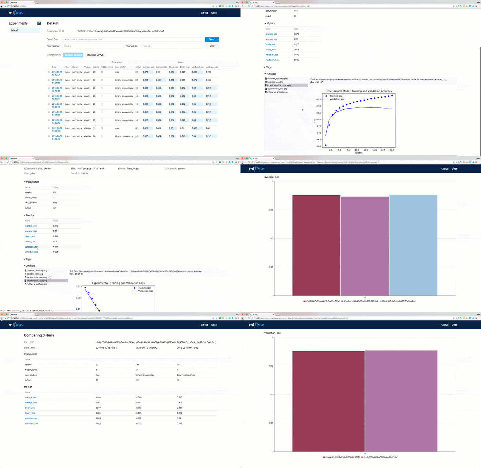
How Tilting Point Does Streaming Ingestion into Delta Lake

$
0
0

Diego Link is VP of Engineering at Tilting Point

Tilting Point is a new-generation games partner that provides top development studios with expert resources, services, and operational support to optimize high quality live games for success. Through its user acquisition fund and its world-class technology platform, Tilting Point funds and runs performance marketing management and live games operations to help developers achieve profitable scale.

At Tilting Point, we were running daily / hourly batch jobs for reporting on game analytics. We wanted to make our reporting near real-time and make sure that we get insights in 5 to 10 mins. We also wanted to make our in-game live-ops decisions based on real-time player behavior for giving real time data to a bundles and offer system, provide up-to-the-minute alerting on LiveOPs changes that actually might have unforeseen detrimental effects and even alert on service interruptions in game operations. Additionally, we had to store encrypted Personally Identifiable Information (PII) data separately for GDPR purposes.

How data flows and associated challenges

We have a proprietary SDK that developers integrate with to send data from game servers to an ingest server hosted in AWS. This service removes all PII data and then sends the raw data to an Amazon Firehose endpoint. Firehose then dumps the data in JSON format continuously to S3.

To clean up the raw data and make it available quickly for analytics, we considered pushing the continuous data from Firehose to a message bus (e.g. Kafka, Kinesis) and then use Apache Spark’s Structured Streaming to continuously process data and write to Delta Lake tables. While that architecture sounds ideal for low latency requirements of processing data in seconds, we didn’t have such low latency needs for our ingestion pipeline. We wanted to make the data available for analytics in a few minutes, not seconds. Hence we decided to simplify our architecture by eliminating a message bus and instead using S3 as a continuous source for our structured streaming job. But the key challenge in using S3 as a continuous source is identifying files that changed recently.

Listing all files every few minutes has 2 major issues:

  • Higher latency: Listing all files in a directory with a large number of files has high overhead and increases processing time.
  • Higher cost: Listing lot of files every few minutes can quickly add to the S3 cost.

Leveraging Structured Streaming with Blob Store as Source and Delta Lake Tables as Sink

To continuously stream data from cloud blob storage like S3, we use Databricks’ S3-SQS source. The S3-SQS source provides an easy way for us to incrementally stream data from S3 without the need to write any state management code on what files were recently processed. This is how our ingestion pipeline looks:

  • Configure Amazon S3 event notifications to send new file arrival information to SQS via SNS.
  • We use the S3-SQS source to read the new data arriving in S3. The S3-SQS source reads the new file names that arrived in S3 from SQS and uses that information to read the actual file contents in S3. An example code below:
spark.readStream \
  .format("s3-sqs") \
  .option("fileFormat", "json") \
  .option("queueUrl", ...) \
  .schema(...) \
  .load()
  • Our structured streaming job then cleans up and transforms the data. Based on the game data, the streaming job uses the foreachBatch API of Spark streaming and writes to 30 different Delta Lake tables.
  • The streaming job produces lot of small files. This affects performance of downstream consumers. So, an optimize job runs daily to compact small files in the table and store them as right file sizes so that consumers of the data have good performance while reading the data from Delta Lake tables. We also run a weekly optimize job for a second round of compaction.


Architecture showing continuous data ingest into Delta Lake Tables

The above Delta Lake ingestion architecture helps in the following ways:

  • Incremental loading: The S3-SQS source incrementally loads the new files in S3. This helps quickly process the new files without too much overhead in listing files.
  • No explicit file state management: There is no explicit file state management needed to look for recent files.
  • Lower operational burden: Since we use S3 as a checkpoint between Firehose and structured streaming jobs, the operational burden to stop streams and re-process data is relatively low.
  • Reliable ingestion: Delta Lake uses optimistic concurrency control to offer ACID transactional guarantees. This helps with reliable data ingestion.
  • File compaction: One of the major problems with streaming ingestion is tables ending up with a large number of small files that can affect read performance. Before Delta Lake, we had to setup a different table to write the compacted data. With Delta Lake, thanks to ACID transactions, we can compact the files and rewrite the data back to the same table safely.
  • Snapshot isolation: Delta Lake’s snapshot isolation allows us to expose the ingestion tables to downstream consumers while data is being appended by a streaming job and modified during compaction.
  • Rollbacks: In case of bad writes, Delta Lake’s Time Travel helps us rollback to a previous version of the table.

Conclusion

In this blog, we walked through our use cases and how we do streaming ingestion using Databricks’ S3-SQS source into Delta Lake tables efficiently without too much operational overhead to make good quality data readily available for analytics.

--

Try Databricks for free. Get started today.

The post How Tilting Point Does Streaming Ingestion into Delta Lake appeared first on Databricks.

New videos from Databricks Academy: Introduction to Natural Language Processing—Latent Semantic Analysis

$
0
0

Databricks’ commitment to education is at the center of the work we do. Through Instructor-Led Training, Certification, and Self-Paced Training, Databricks Academy provides strong pathways for users to learn Apache Spark™ and Databricks to push their knowledge to the next level.

Our latest offering is a series of short videos introducing the Natural Language Processing technique, Latent Semantic Analysis (LSA). This series explains the conceptual framework of the technique and how the Databricks Runtime for Machine Learning can be used to apply the technique to a body of text documents using Scikit-Learn and Apache Spark.

If you’d like to follow along with the videos on your own computer, simply download the Databricks notebook. If you don’t have a Databricks account yet, get started for free on Databricks Community Edition.

If you’d like to dive deeper into Machine Learning using Databricks, check out our self-paced course Introduction to Data Science and Machine Learning / AWS (also available on Azure) at Databricks Academy.

Introduction to Latent Semantic Analysis

This video introduces the core concepts in Natural Language Processing and the Unsupervised Learning technique, Latent Semantic Analysis (LSA). The purposes and benefits of the technique are discussed. In particular, the video highlights how the technique can aid in gaining an understanding of latent, or hidden, aspects of a body of documents—in addition to reducing the dimensionality of the original dataset.

A Trivial Implementation of LSA using Scikit-Learn

This video introduces the steps in a full LSA Pipeline and shows how they can be implemented in Databricks Runtime for Machine Learning using the open-source libraries Scikit-Learn and Pandas.

These steps are:

This video uses a trivial list of strings as the body of documents so that you can compare your own intuition to the results of the LSA. After completing the process, we examine two byproducts of the LSA—the dictionary and the encoding matrix—in order to gain an understanding of how the documents are encoded in topic space.

A Second LSA

Here we work through the same steps from the previous video in a second full LSA Pipeline, once more in Databricks Runtime for Machine Learning using the open-source libraries Scikit-Learn and Pandas.

This video uses a slightly more complicated the body of documents: strings of text from two popular children’s books. After completing the process, we examine two byproducts of the LSA—the dictionary and the encoding matrix—in order to gain an understanding of how the documents are encoded in topic space. Finally, we plot the resulting documents in their topic-space encoding using the open source library Matplotlib.

Improving the LSA with a TFIDF

This video works through a third full LSA Pipeline using Databricks’ Runtime for Machine Learning and the open-source libraries Scikit-Learn and Pandas.

Here we iterate on the previous LSA Pipeline by using an alternate method, Term Frequency-Inverse Document Frequency, to prepare the Document-Term Matrix. After completing the process, the video examines two byproducts of the LSA—the dictionary and the encoding matrix—in order to gain an understanding of how the documents are being encoded in topic space. Finally, the video plots the resulting documents in their topic-space encoding using the open source library Matplotlib and compares the plot to the plot prepared in the previous video.

Latent Semantic Analysis with Apache Spark

In this video, we begin looking at a new, larger dataset: the 20 newsgroups dataset. In order to work with this larger dataset, we move the analysis pipeline to Apache Spark using the Scala programming language. This video introduces a new type of NLP-specific preprocessing: lemmatization. We also discusses key differences between performing NLP in Scikit-Learn and Apache Spark.

We hope that you find these videos informative, as well as entertaining! The full video playlist is here. If you’d like to dive deeper into Machine Learning using Databricks, check out our self-paced course Introduction to Data Science and Machine Learning / AWS (also available on Azure) at Databricks Academy,


--

Try Databricks for free. Get started today.

The post New videos from Databricks Academy: Introduction to Natural Language Processing—Latent Semantic Analysis appeared first on Databricks.
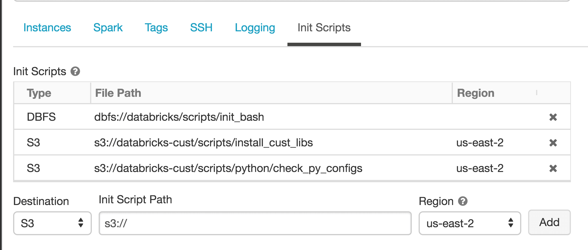
Databricks and Informatica Accelerate Development and Complete Data Governance for Intelligent Data Pipelines

$
0
0

The value of analytics and machine learning to organizations is well understood. Our recent CIO survey showed that 90% of organizations are investing in analytics, machine learning and AI. But we’ve also noted that the biggest barrier is getting the right data in the right place and in the right format. So we’ve partnered with Informatica to enable organizations to achieve more success by enabling new ways to discover, ingest and prepare data for analytics.

Ingesting Data Directly Into Delta Lake

Getting high volumes of data from hybrid data sources into a data lake in a way that is reliable and high-performant is difficult. Datasets are often dumped in unmanaged data lakes with no thought of a purpose. Data is dumped into data lakes with no consistent format, making it impossible to mix reads and appends. Data can also be corrupted in the process of writing it to a data lake, as writes can fail and leave partial datasets.

Informatica Cloud Data Ingestion (CDI) enables ingestion of data from hundreds of data sources. By integrating CDI with Delta Lake, a smart ingestion can take place with the benefits of Delta Lake. ACID transactions ensure that writes are complete, or are backed out if they fail, leaving no artifacts. Delta Lake schema enforcement ensures that the data types are correct and required columns are present, preventing bad data from causing data corruption. The seamless integration between Informatica CDI and Delta Lake enables data engineers to quickly ingest high volumes of data from multiple hybrid sources into a data lake with high reliability and performance

Preparation

Every organization is limited in resources to format data for analytics. Ensuring the datasets can be used in ML models requires complex transformations that are time consuming to create. There are not enough highly skilled data engineers available to code advanced ETL transformations for data at scale. Furthermore, ETL code can be difficult to troubleshoot or modify.

The integration of Informatica Big Data Management (BDM) and the Databricks Unified Analytics Platform makes it easier to create high-volume data pipelines for data at scale. The drag and drop interface of BDM lowers the bar for teams to create data transformations by removing the need to write code to create data pipelines. And the easy to maintain and modify pipelines of BDM can leverage the high volume scalability of Databricks by pushing that work down for processing. The result is faster and lower cost development of high-volume data pipelines for machine learning projects. Pipeline creation and deployment is increased 5x, and pipelines are easier to maintain and troubleshoot.

Discovery

Finding the right datasets for machine learning is difficult. Data scientists waste precious time looking for the right datasets for their models to help solve critical problems. They can’t identify which datasets are complete and properly formatted, and have been properly verified for usage as the correct datasets.

With the integration of Informatica Enterprise Data Catalog (EDC) with the Databricks Unified Analytics Platform, Data Scientists can now find the right data for creating models and performing analytics. Informatica’s CLAIRE engine uses AI and machine learning to automatically discover data and make intelligent recommendations for data scientists. Data scientists can find, validate, and provision their analytic models quickly, significantly reducing the time to value. Databricks can run ML models at unlimited scale to enable high-impact insights. And EDC can now track data in Delta Lake as well, making it part of the catalog of enterprise data.

Lineage

Tracing the lineage of data processing for analytics has been nearly impossible. Data Engineers and Data Scientists can’t provide any proof of lineage to show where the data came from. And when data is processed for creating models, identifying which version of a dataset, model, or even which analytics frameworks and libraries were used has become so complex it has moved beyond our capacity for manual tracking.

With the integration of Informatica EDC, along with Delta Lake and MLflow running inside of Databricks, Data Scientists can verify lineage of data from the source, track the exact version of data in the Delta Lake, and track and reproduce models, frameworks and libraries used to process the data for analytics. This ability to track Data Science decisions all the way back to the source provides a powerful way for organizations to be able to audit and reproduce results as needed to demonstrate compliance.

We are excited about these integrations and the impact they will have on making organizations successful, by enabling them to automate data pipelines and provide better insights into those pipelines. For more information, register for this webinar https://dbricks.co/INFA19.


--

Try Databricks for free. Get started today.

The post Databricks and Informatica Accelerate Development and Complete Data Governance for Intelligent Data Pipelines appeared first on Databricks.

Databricks is a Diamond Partner at Snowflake Summit

$
0
0

Here at Databricks, we are excited to participate in the first Snowflake Summit as a Diamond Partner. The event takes place June 3-6 at the Hilton San Francisco Union Square and is another great opportunity to share how Databricks and Snowflake have partnered together to provide:

  • Massively scalable data pipelines. Pipelines running on Databricks can combine batch and streaming data and are up to 100x faster than OSS Apache Spark, lowering your total cost of ownership.
  • High scale concurrent access to data. Data is written to Snowflake, the Data Warehouse for the cloud where it can be accessed at high concurrency for BI, reporting and visualization tools.
  • Powerful machine learning insights. Databricks, a Unified Analytics Platform, can access data in Snowflake to run machine learning jobs, and write the results back into Snowflake. Data analysts can access those machine learning results for deeper insights and better decisions.

The Snowflake Summit is full of customer presentations to hear and learn from, with three sessions featuring joint Databricks and Snowflake customers.  Check these out to see our customers speak directly about their results:

  • Chesapeake Energy is augmenting real-time IOT streams with machine learning techniques to explore historical IOT data (Tuesday June 4th 1.55-2.15 PM PDT)
  • Talroo migrated from MySQL to Snowflake and Databricks with impressive results. They automated data pipelines and saw a 10x improvement in their volume of machine learning insights (Tuesday June 4th 2.30-3.15 PM PDT)
  • ShopRunner automated data pipelines to feed Snowflake and drive machine learning with Databricks. Their machine learning results drive a retail recommendation engine that can visually match and suggest apparel (Tuesday June 4th 3:30pm-4:15pm PM PDT)

We look forward to seeing you at Snowflake Summit.  Please stop our Booth #D2 to see examples of the integration between the Databricks Unified Analytics Platform and Snowflake, or visit our webpage at www.databricks.com/snowflake for more information and customer stories.


--

Try Databricks for free. Get started today.

The post Databricks is a Diamond Partner at Snowflake Summit appeared first on Databricks.

Viewing all 1999 articles
Browse latest View live